Sparse MLP Distillation

post by slavachalnev · 2024-01-15T19:39:02.926Z · LW · GW · 3 comments

Contents

  TLDR
  Introduction
  Training Setup
  Two Types of Features
  Activation Monosemanticiy
  Downsides of Sparse Distillation
  Conclusion
  Appendix A: The Neuron Simulator Encoder vs Decoder Mystery
  Appendix B - ReLU vs GELU
  Appendix C: Layer 0 MLP Results
None
3 comments

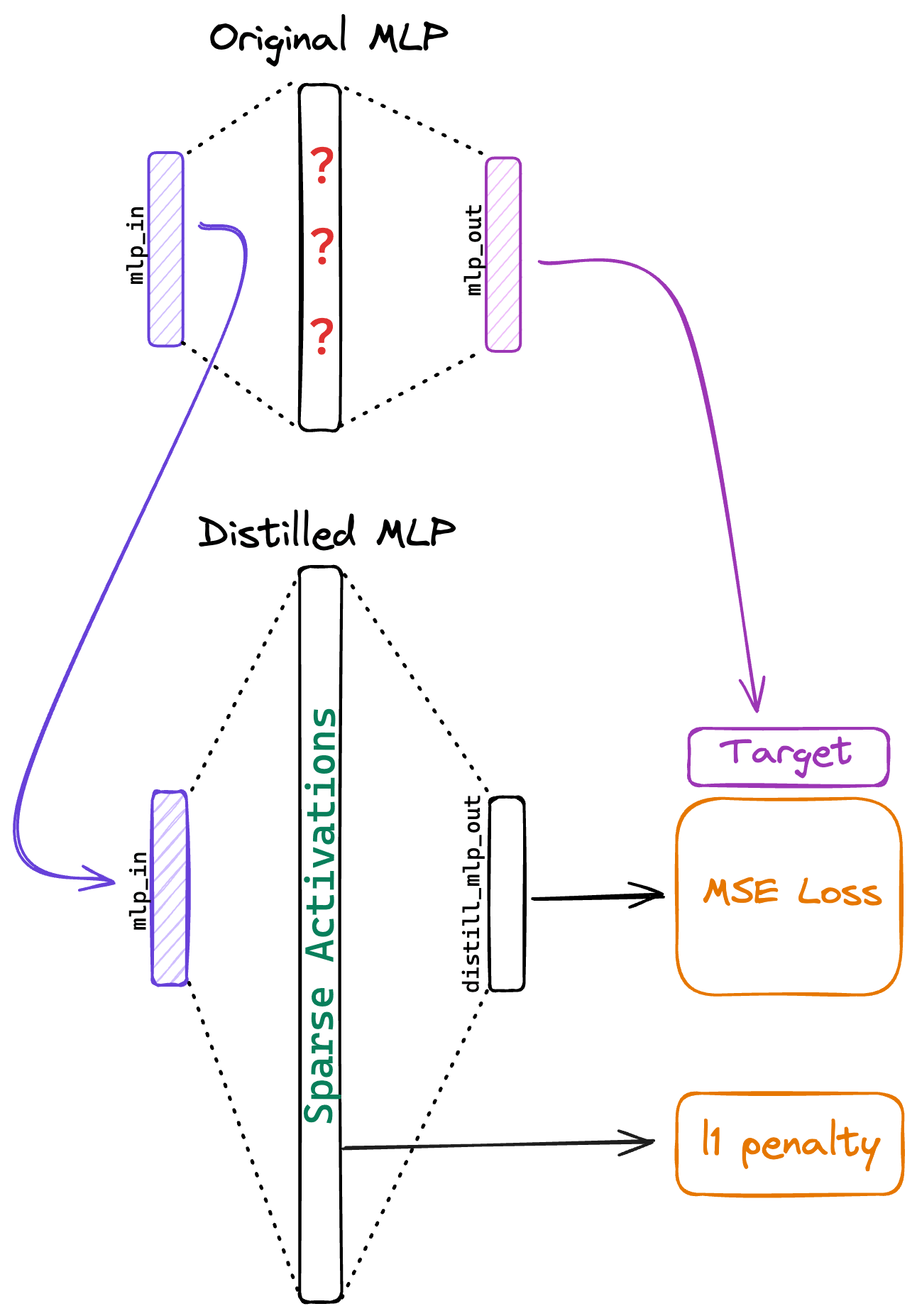
This is a research report about my attempt to extract interpretable features from a transformer MLP by distilling it into a larger student MLP, while encouraging sparsity by applying an L1 penalty to the activations, as depicted in Figure 1. I investigate the features learned by the distilled MLP, compare them to those found by an autoencoder, and discuss limitations of this approach.

See the code here: https://github.com/slavachalnev/ft_exp. A large part of both the training and analysis code is adapted from Neel Nanda's SAE replication.

TLDR

I find that a subset of the distilled MLP's neurons act as 'neuron simulators', mimicking the activations of the original MLP, while the remaining features are sparse and somewhat monosemantic. Unfortunately, the distilled model is not as good as an autoencoder in terms of activation monosemanticity and reconstruction error.

 

Introduction

The hidden layer neurons in transformer multilayer perceptrons (MLPs) are polysemantic, making them hard to interpret. The neuron activations are an intermediate state in the computation of the MLP's function. I wish to extract interpretable features out of this intermediate state to learn about what the MLP is doing.

One method for extracting features out of transformer MLPs is to train a sparse autoencoder on the activations. However, the autoencoder may learn features of the activation distribution which are not relevant to the function a particular MLP is performing. I explore an alternative method which, if successful, would allow us to find interpretable features that are directly useful for computing the function of a specific MLP.

The idea is to 'refactor' the MLP such that it retains its original function but with sparse activations in the hidden layer. To do this, I distill the original MLP into a new MLP, while imposing a sparsity constraint. My reasoning is that if two MLPs have the same input-output behaviour, then they are likely 'doing the same thing' and using the same features.

To compensate for the loss of expressiveness due to sparsity, the distilled MLP has an expanded hidden layer, containing more neurons than the original MLP. Importantly, the new MLP is trained to duplicate the original MLP's behaviour, without learning new or unrelated features.

 

Training Setup

The model I distill and investigate throughout this report is the second layer MLP of the tiny-stories-2L-33M transformer. I run it over the roneneldan/TinyStories dataset, using transformer_lens to record pre- and post- MLP activations.

Student model details:

• Standard MLP with one hidden layer.
• Hidden layer dimension is 4x larger than the original MLP's hidden layer.
• ReLU activation function (See Appendix B for discussion).
• Decoder weights are normalised to 1.

The student MLP is trained to predict the original MLP's outputs given the inputs. We use mean squared error loss with an L1 penalty on the hidden layer activations to promote sparsity, specifically, $\text{loss}=\text{MSE}+\lambda \sum \left(\text{activations}\right)$, where the L1 penalty coefficient $\lambda$ is set to $2\times {10}^{-4}$ unless otherwise specified. We train in-distribution for $4\times {10}^9$ tokens, using Adam, weight decay, a learning rate of $5\times {10}^{-5}$ with a cosine decay schedule.

 

Two Types of Features

What does the new model end up learning?

First, let's check if any of the new model's neurons are similar to the original MLP's neurons. For every neuron in the new model, we find the closest original neuron by cosine similarity of the decoder vectors^[1].

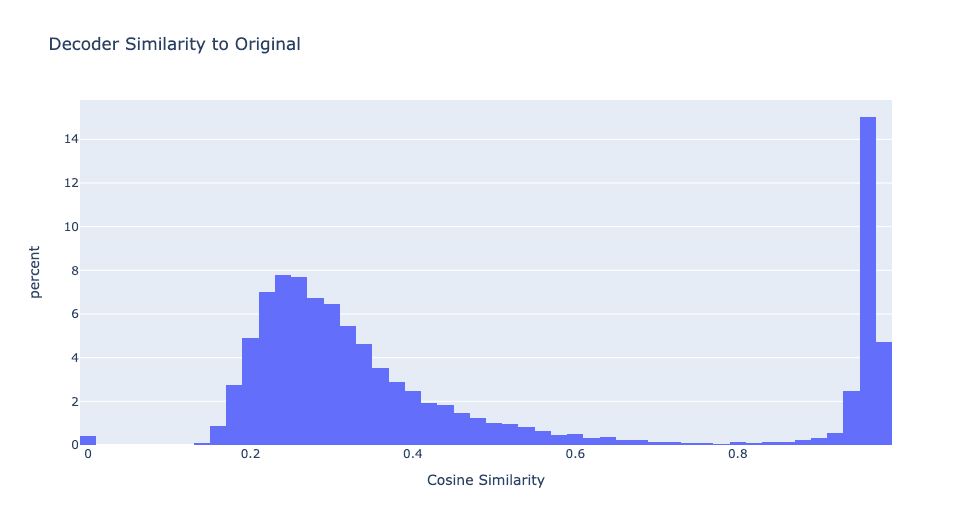
29% of the features have very high cosine similarity with the original MLP's decoder. Since the student model has four times as many neurons as the original model, this means there is approximately one high similarity neuron for every original neuron. Figure 2 depicts the distribution of cosine similarities between each neuron in the distilled model and the closest original model neuron.

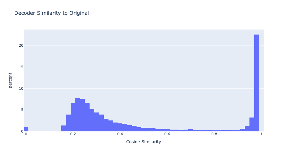
As we will see, these two types of features have very different properties and it is useful to separate them. Let's name these two types of features "neuron simulators" and "sparse features" and define a feature to be a "neuron simulator" if it's max decoder similarity is greater than 0.8. Otherwise, it is a "sparse feature".

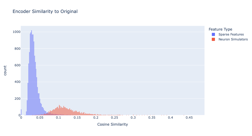
We defined feature type by similarity of the decoder vectors. However, if we plot encoder similarity, as shown in Figure 3, we see a notably different distribution.

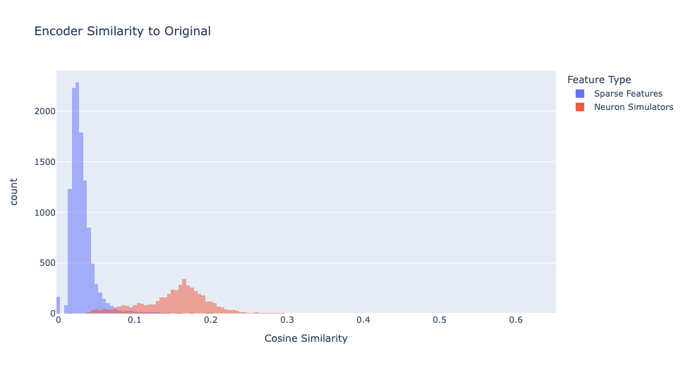
Even though the decoders match almost perfectly, the encoder vectors only have a modest cosine similarity (with a mean of 0.1538 and a standard deviation of 0.0475). I think this happens because a neuron's encoder vector is harder to learn since the neuron activates on a wide distribution of data, while the decoder is easier to learn because when the neuron is activated, it always writes in a single direction. See Appendix A for details.

Plotting the frequency of neuron activations in Figure 4, we see that the activation frequencies of sparse features and neuron simulators are clearly distinct. The neuron simulators activate much more frequently than sparse features.

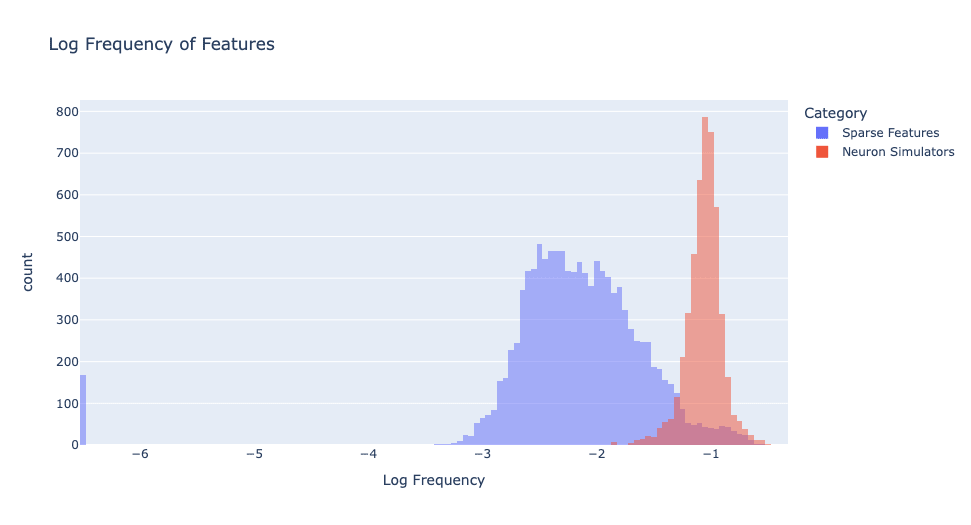
As we will see in the next section, sparse features are considerably more monosemantic and understandable than neuron simulators. We want our distilled model to be sparse and interpretable, so we want it to consist of sparse features, not neuron simulators.

In Figure 5 we mean-ablate each type of feature in order to see the relative importance of sparse features vs neuron simulators for various L1 penalty coefficients.

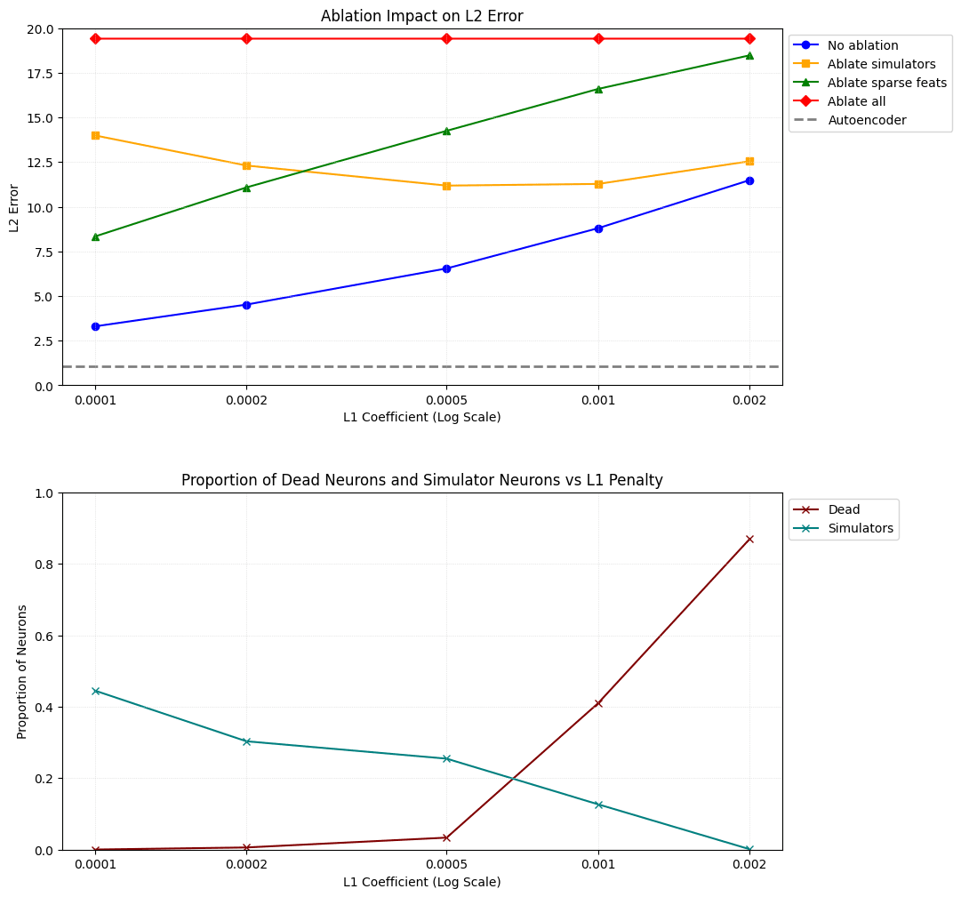
The blue line in the top plot of Figure 5 represents the reconstruction error of the full model without any ablations. As expected, it consistently goes up as we increase L1 penalty. We see that even the model with the lowest L1 penalty still has a reconstruction error of  3.3038, more than three times greater than that of the autoencoder with an error of just 1.0808!

The yellow line represents the reconstruction error when relying exclusively on sparse features. As we increase the L1 penalty, the sparse features capture more of the original model's behaviour up until a point somewhere between L1=0.0005 and L1=0.001, where the reconstruction error goes back up because neurons start to die and we actually get fewer sparse features (as you can see in the bottom plot of Figure 5.)

So not only does the distilled model not capture as much of the original model's signal compared to the autoencoder, but most of the 'work' is done by the neuron simulators, thus leaving most of the functionality of the MLP unexplained. It looks like we can't fix this by increasing the L1 penalty, as this results in even higher reconstruction error and more dead neurons.
 

Activation Monosemanticiy

Inspecting top activating examples of the distilled model neurons reveals that many of the neurons are monosemantic. There is a large difference in monosemanticity between the activations of neuron simulators and sparse features. Sparse features look much more interpretable, while neuron simulators are, as expected, no better than the original model's neurons.

Figure 6 shows the top activating examples of neuron 2, which is the first interpretable sparse feature (neuron 0 is also a sparse feature but is not monosemantic, and neuron 1 is dead). This feature activates on the word 'important' in the context of learning a valuable lesson.

I inspected the top activations for the first 50 neurons of both the distilled model and an autoencoder trained on the same model and dataset.

The autoencoder was trained by Lucia Quirke and Lovis Hendrich, who kindly let me use it. It was trained for $5\times {10}^8$ tokens with an L1 coefficient of $1.2\times {10}^{-6}$, a square root activation penalty, and weight decay. It has a hidden dimension of 16384, the same as the distilled model.

For every neuron, I select the top activating examples and I try to come up with a clear rule which would explain the activations. I score each neuron by how monosemantic the activations are according to a grading rubric. You can look at the activations here, and my ratings here.

 

Model	Average Score
Distilled model (neuron simulators)	1.154
Distilled model (sparse features)	2.833
Autoencoder	3.176

Table 1. Interpretability score on a scale of 0 to 4.

We see that there is a large difference in monosemanticity between neuron simulators and sparse features, while autoencoder features are the most monosemantic.

Anecdotally, I have found that features with large max activation values seem more interpretable than features which don't activate as strongly.

 

Downsides of Sparse Distillation

We see from Figure 5 and Table 1 respectively, that the distilled model does not compare favourably to the autoencoder in terms of both reconstruction error and activation monosemanticity. The reconstruction error is particularly bad when we remove the neuron simulators either by ablation or by increasing the L1 penalty. So even though the number of active autoencoder features is approximately equal to the number of sparse features of the distilled model, it looks like the autoencoder's features are higher quality.

There is also a conceptual problem with the distillation approach: MLPs don’t function in isolation! Just as features are not aligned with individual neurons in an single MLP, features may be spread over neurons in multiple consecutive MLPs. Studying individual MLPs in isolation doesn't necessarily carve reality at the joints. Thus, both the distillation and the autoencoder approaches may have trouble picking up multi-layer features.

This is where the autoencoder approach has an advantage over distillation. If we take the view of features as directions, then even multi-layer features must eventually materialise as some direction in the residual stream, so that they can be picked up and used by a later component.

This means that an autoencoder, trained to represent residual stream activations, should be able to pick up multi-layer features which have appeared up to that point in the model. So if we train one such residual stream autoencoder for each layer of the transformer, we should be able to see multi-layer features gradually appear as they are built up by the model.

Unfortunately, I see no similarly clear way of using sparse MLP distillation to capture multi-layer features.

 

Conclusion

Even though I like the idea of 'refactoring' an MLP with sparse distillation it turns out to be worse than an autoencoder at extracting interpretable features. Furthermore, due to the focus on a single MLP, sparse distillation may miss multi-layer features.

Further questions to look into:

• What kinds of features are learned by distillation vs autoencoder?
• As we increase the L1 penalty, what's the mechanism for the change in importance of sparse features vs neuron simulators, and what functionality remains in the neuron simulators?
• If we increase the size of the student model sufficiently, do we end up with compelling features?

---

I would like to thank Evan Hockings for valuable feedback on a draft of this post. I would also like to thank Lucia Quirke and Lovis Hendrich for letting me use an autoencoder they trained.

---

 

Appendix A: The Neuron Simulator Encoder vs Decoder Mystery

Taking a look at the neuron simulator features, we see that while the decoder vectors point in the same direction as the original model's neurons (> 0.9 cosine similarity), the encoder only matches with a modest cosine similarity of around 0.1 to 0.2.

Why is there an almost perfect decoder match, but only approximate encoder match?

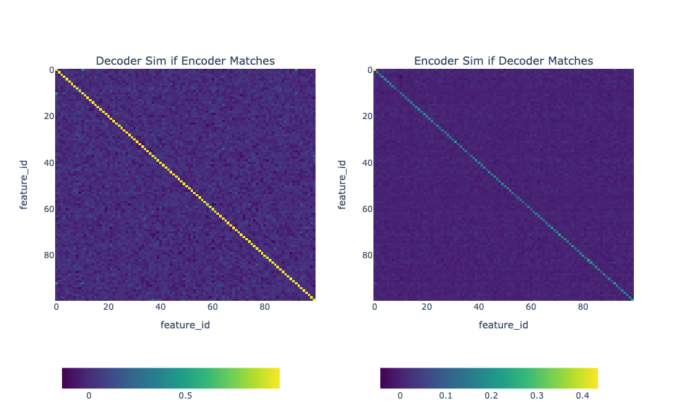
We should first check to make sure that each neuron simulator matches a single neuron. One way to do this is to ask "if the encoder of feature $i$ matches neuron $j$, do the decoders also match?" We see in Figure 7 that they do match: if the decoder of a feature is close to a particular neuron, then that neuron's encoder will be close to the same feature.

Despite the low cosine similarity, the neuron simulator features are nonetheless highly correlated with the neuron they are simulating. Figure 8 is a plot of activations of the first simulator neuron against the neuron it is simulating. The correlation coefficient is 0.98865.

I suspect that for every neuron we are simulating, the encoder vector is harder to learn because it activates on a wide distribution of data, while the decoder always writes in one specific direction.

To test this hypothesis, I constructed a toy setup with a 1000-dimensional normally distributed input and an original MLP with just a single neuron which writes to a single output direction. We then train a new MLP, also with a single neuron, to predict the outputs of the original.

We see in Figure 9 that the decoder converges quickly, while the encoder does not converge at all. The encoder's cosine similarity fluctuates around 0.3, which is not dissimilar to the encoder similarity distribution in Figure 3.

We should also check to make sure that this effect is not a quirk of forcing the decoder L2 norms to be at most 1. Removing this constraint and letting the decoder vectors have any length, we see in Figure 10 that the encoder similarity does eventually reach 1 but it converges much more slowly than the decoder.

So the low similarity of the encoder vectors is only partially due to the decoder norms being capped at 1.

Note that these single-neuron results are sensitive to learning rate and input dimension hyperparameters. You can read the (very basic) implementation here.

This explanation still leaves me confused about why the decoders of sparse features have moderately high cosine similarity with the original model.

 

Appendix B - ReLU vs GELU

Even though the original model's activation function is GELU, the distilled model instead uses ReLU in the above experiments.

Training with ReLU makes the activations easier to think about. The higher the activation, the more the feature is present. GELU, on the other hand, can be negative and has unintuitive behaviour around 0.

Additionally, using GELU causes most features to be neuron simulators, as shown in Figure 11.

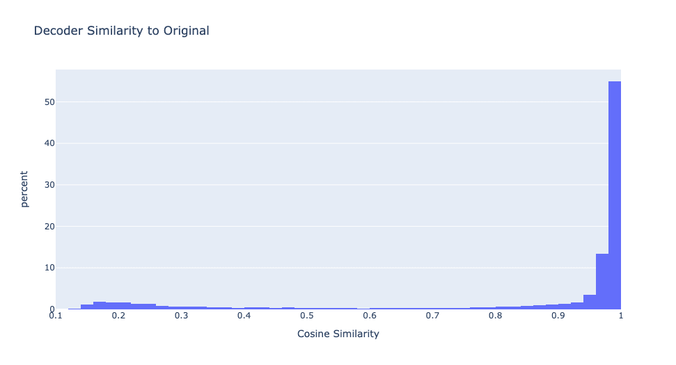
70% of the features are simulating original MLP neurons, while the remaining sparse features are almost dead. This is with an L1 coefficient of 0.0002, same as the main ReLU model I investigate above.

Interestingly, both encoder and decoder vectors tend to form clusters, typically in pairs or triplets, so that each neuron in the original MLP is simulated by two or three very similar neurons.

 

Appendix C: Layer 0 MLP Results

All of the findings above are for the second layer MLP of the tiny-stories-2L-33M transformer. If, instead, we distill the first layer MLP, we see that the similarity and the frequency distributions look similar.

---

1. ^{^}

   A note on my use of 'encoder' and 'decoder'. The MLP is computed as:

   $\text{MLP}\left(x\right)=W_2\left(\text{ReLU}\right(W_{1}x+b_1\left)\right)+b_2$

   I refer to the rows of $W_1$ as encoder vectors and the columns of $W_2$ as decoder vectors. So each neuron has an encoder and a decoder vector of size $d_{model}$, and there are $d_{mlp}$ neurons.

3 comments

Comments sorted by top scores.