Finding Skeletons on Rashomon Ridge
post by David Udell, Peter S. Park, NickyP (Nicky) · 2022-07-24T22:31:59.885Z · LW · GW · 2 commentsContents
  Introduction
  Loss Landscapes and Rashomon Ridges
  Skeletons
  Skeleton Hunting
    Functioning Machinery under Continuous Deformation
    L1 Regularization and Pruning
  Experimental Results
None
2 comments
A product of a SERI MATS research sprint (taking 1.5 weeks).
Cannot yet assign positively to animal or vegetable kingdom, but odds now favour animal. Probably represents incredibly advanced evolution of radiata without loss of certain primitive features. Echinoderm resemblances unmistakable despite local contradictory evidences. Wing structure puzzles in view of probable marine habitat, but may have use in water navigation. Symmetry is curiously vegetable-like, suggesting vegetable’s essentially up-and-down structure rather than animal’s fore-and-aft structure …
Vast field of study opened … I’ve got to dissect one of these things before we take any rest.
--H. P. Lovecraft, At the Mountains of Madness
Introduction
This is our MATS research-sprint team's crack at working towards the True Name (the formalization robust to arbitrary amounts of adversarial optimization power) [LW · GW] of a model's "internal machinery."
Some weights and neurons in a model are essential to its performance, while other weights and neurons are unimportant. Our idea is that, ontologically, the True Name of a model's internal machinery is its subnetwork of important weights and neurons -- its "skeleton." This subnetwork is still a (sparser) model, but hopefully a far more interpretable model than the original.
What makes this a theoretically interesting True Name is our theory's intersection with the theory of "broad peaks" ('Rashomon ridges) in the loss landscape of overparametrized models. [LW · GW] Rashomon ridges suggest that different overparametrized models, trained to optimality on the same task, will share a single skeleton. Furthermore, Rashomon ridges suggest a means to compute the shared skeleton of that class of models.
We were able to execute our pruning algorithm effectively by leaning on regularization. -regularization-plus-pruning-extremely-small-weights shrunk models significantly while never unacceptably varying loss or accuracy. However, the models we trained did not obviously converge to skeletons, as measured by their losses on an off-distribution task. This means something is up with one or more of our premises: (1) Rashomon ridges are not so naively traversable and/or (2) our argument for shared internal machinery amongst models on a Rashomon ridge fails.
Loss Landscapes and Rashomon Ridges
A loss landscape is a geometric representation of how good various models are at a task.
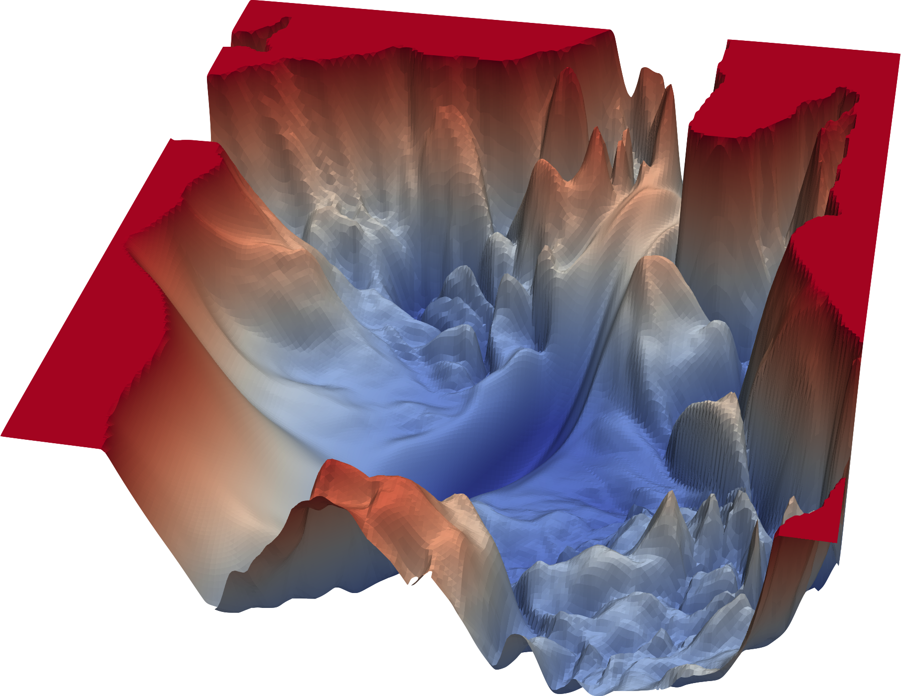
coordinates in the loss landscape above represent models with two parameters, and . Thus, the two horizontal dimensions of the loss landscape represents a model space -- every point in that plane is a possible model you could have. For larger models, their model spaces will have correspondingly more dimensions.
The vertical dimension in the loss landscape represents how good the model is at a given task. (Whether we represent this as higher-is-better or lower-is-better is immaterial.) In the above loss landscape, then, every point represents a model and its loss. SGD initializes at some random point in that landscape, and rolls downhill from there, "reaching optimality" once the model settles into some rut.
A Rashomon manifold (or Rashomon ridge) is a large flat plateau in the loss landscape of overparameterized optimal models. It has been conjectured that, [LW · GW] and disputed [LW(p) · GW(p)] whether [LW(p) · GW(p)], these overparametrized models trained to optimality land on Rashomon manifolds that encompass all optima. Rashomon ridges are conjectured to widen and narrow periodically, and to run through all the optima in overparameterized model spaces. (The idea here is that overparameterized models have a lot of free, superfluous parameters, and that these free dimensions in model space almost certainly allow all optima in the high-dimensional loss landscape to intersect each other.)
Skeletons
One can imagine an optimal model additionally barnacled with superfluous neurons, where all the weights in the superfluous neurons are zero. These zeroed-out neurons don't help or hurt the model's loss -- they just sit there, inert. We can therefore permanently prune these zeroed-out neurons from the model without changing the model's loss.
Consider only those weights and neurons that would counterfactually tank a model's loss were they pruned (ignoring the irrelevant weights and neurons in the model). Call this sparse subnetwork of important weights and neurons the model's skeleton.
Because this subnetwork is plausibly much smaller than the original network, it will be correspondingly easier to interpret with existing techniques. The challenge now lies, of course, in finding an arbitrary optimal model's skeleton.
Skeleton Hunting
Functioning Machinery under Continuous Deformation
Overparametrized models trained to optimality (possibly) sit on a Rashomon ridge of related models. When you move from one model to its neighbor on the Rashomon ridge, you're looking at some small change in model weights that doesn't change the model's loss. So traveling around on the Rashomon ridge means seeing a model continuously morph, Shoggoth-like, into models with equivalent losses via small changes. You can morph the model in all sorts of ways by moving around the Rashomon ridge, but you never (1) discontinuously morph it or (2) hurt its loss.
Because all these changes are small and the loss is held constant, whatever machinery the model is using internally cannot be being radically revised. If step sizes were large, we could jump from a model that succeeds one way to a model that succeeds in a very different way, stepping over a valley of hybrid, non-functional models in between. If model losses were allowed to vary, then travel through the valley of non-functional hybrid models would be permitted. But when step sizes are kept small, so that the model is only ever being altered in small ways, and when losses are held constant or nearly constant, keeping the model on a flat Rashomon plateau, we bet the model's internal machinery cannot change.[1]
We leverage the fact that all the models of a Rashomon ridge then share their internal machinery -- "skeleton" -- to actually construct the skeleton of an arbitrary model on that ridge! What we're after is an exposed skeleton: the sparsest model on the Rashomon ridge. Because all models on the ridge share a skeleton, locating this exposed-skeleton model gives us insight into the inner workings of all other models on the ridge.
Our method is to (1) apply regularization to the optimal models, and then (2) prune all the extremely small weights of those models. We found that this surprisingly did not significantly alter model losses or accuracy, and resulted in substantially smaller, equivalently powerful models -- our skeletons.
Regularization and Pruning
How can we prune in a manner that never significantly moves the model's loss? A common way to train a model simultaneously towards optimality and low-dimensionality (a model with many zero weights) is regularization. If denotes the loss function (on the weight space ) given by the training dataset, then regularization denotes the technique of applying SGD not on itself, but on the modified loss function
for some Here, the function is the norm of the weight vector . The weight should ideally be not so small that the regularization has essentially no effect, but not so large that training ceases to care about model optimality.
regularization drives many weights to decrease in magnitude to zero while maintaining an optimal model. Intuitively, regularization reduces the magnitude of all the weights by a fixed positive amount (corresponding to the slope of the absolute value function), until weights are set to zero.
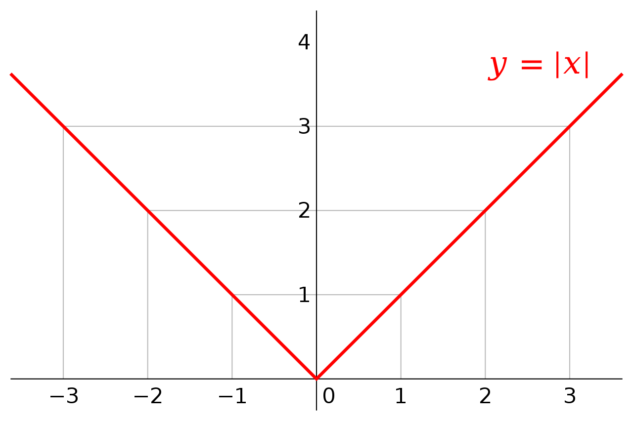
Once regularization has driven down the weights sufficiently, we permanently prune out those weights.
Experimental Results
Our plan was to start with two different optimal models, prune each of them, and probe whether they have become more similar as a result. To do so, we need a way to measure the similarity of two neural-net models. No canonical measure of neural network similarity currently exists, however [LW · GW]. Given this, we were inspired by Ding et al. to first look at the comparative behavior of the two models out-of-distribution. This is because neural nets which are canonically similar inside of their respective black boxes would as a consequence behave similarly outside of them. That is, they would have similar behavior on datasets other than the training dataset.
We had predicted that our two models, trained to optimality on the same task, would end up as the same pruned model (or at least highly similar in their network structures). This would be surprising, and not something that other theories would wager would happen!
We trained two separate models to optimality at the CIFAR10 image classification task (sorting 32x32 images of frogs, planes, trains, etc.). We next regularized those two optimal models, so as to incentivize them to drive down the sum of their weights. This never substantially changed their losses or accuracy. Finally, we heavily pruned the two regularized models, permanently deleting all weights below the threshold of 0.05, which we found to not significantly reduce accuracy.
Deploying our image models after pruning them via the above light--regularization-and-pruning on an entirely separate MNIST classification task. Our models had previously inhabited a world of 32x32 images of frogs and planes and so on, and so had never before encountered handwritten digits. Thus, the handwritten digits task probes their out-of-distribution behavior, which isn't constrained by the optimality criterion on in-distribution performance. If the models were the same or were becoming the same as a consequence of pruning, then this unconstrained external comparison of similarity would reveal that. Two truly identical models will behave identically, on and off distribution.
We obtained a variety of optimal models, each of which was obtained by applying a different pruning strategy to either Model 1 or Model 2. Then, for every pair of these pruned models, we computed the cosine similarity of their prediction vectors on the out-of-distribution MNIST dataset
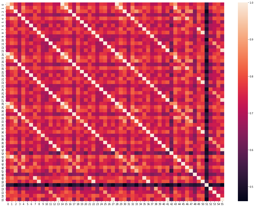
Here's our plot of the cosine similarity of each pair of model's behavior on the out-of-distribution MNIST task:
0: Model 1, trained for 200 epochs, unpruned
1: Model 1, L1 regularization with 1e-6 for 200 epochs
2: Model 1, L1 regularization with 1e-6 for 400 epochs
3: Model 1, L1 regularization with 3e-6 for 300 epochs
4: Model 1, L1 regularization with 1e-5 for 100 epochs
5: Model 1, L1 regularization with 1e-5 for 300 epochs
6: Model 2, trained for 200 epochs, unpruned
7: Model 2, L1 regularization with 1e-6 for 200 epochs
8: Model 2, L1 regularization with 1e-6 for 400 epochs
9: Model 2, L1 regularization with 3e-6 for 300 epochs
10: Model 2, L1 regularization with 1e-5 for 100 epochs
11: Model 2, L1 regularization with 1e-5 for 300 epochs
12: Model trained with L1 Regularization 1e-6, 200 epochs
13: Model trained with L1 Regularization 1e-6, 300 epochs
14-27: same with weights below 0.01 removed
28-41: same with weights below 0.02 removed
42-55: same with weights below 0.05 removed
Unsurprisingly, pruning from a higher weight threshold more dramatically altered out-of-distribution model behavior than pruning only smaller weights did. More epochs spent in regularization produced smaller pruned models with similar out-of-distribution behavior to their unpruned originals.
Our various models all had similarly varied out-of-distribution behavior -- generally, a cosine similarity of >0.6 with each other on MNIST. Model 51 was our only exception to this rule. As you can see above, model 51's cosine similarity of <0.6 (in black/purple) stands out on the plot, and 51 curiously suffered from a relatively degraded loss on CIFAR10 (curiously, because models regularized harder and pruned at the same threshold did not suffer loss degradation in the same way).
Tragically, then, our data does not suggest that models on a Rashomon ridge converge to a shared skeleton under regularization plus pruning.
- ^
The Worry from "Multi-Skeletal" Models:
Consider models with "two skeletons" that each effectively and independently contribute to the loss, but that pass through lossy channels on their way out of the model. This model could smoothly shift between its substantially different skeletons by shifting weight contributions from one skeleton over to the other, such that loss is smoothly preserved. If examples of this exist, then our premise that all optimal models on a Rashomon ridge share a single skeleton would be false.
One reason to worry less about this "multi-skeleton" failure case of our theory is that the trained models we're looking at are already trained to optimality. If the models are optimal, then it shouldn't be that they have a well of optimization power to draw from to keep their loss constant. They can't have a whole second skeleton, held in reserve. Instead, the models should be doing as well as is possible with any small change -- "multi-skeletal" models would be holding back and so would be able to fall further in the loss landscape. This implies that all the machinery of an optimal model is actively in use, and thus that every optimal model is "mono-skeletal."
2 comments
Comments sorted by top scores.
comment by Charlie Steiner · 2022-07-25T00:14:47.643Z · LW(p) · GW(p)
I don't see why you dismiss multi-skeletal models. If your NN has a ton of unused neurons, why can't you just deform those unused neurons to an entirely different model, them smoothly turn the other model on while turning the original off? Sure, you'd rarely learn such an intermediate state with SGD, but so what? The loss ridge is allowed to be narrower sometimes.
Replies from: Peter S. Park↑ comment by Peter S. Park · 2022-07-26T03:39:25.053Z · LW(p) · GW(p)
Thanks so much for your insightful comment, Charlie! I really appreciate it.
I think you totally could do this. Even if it is rare, it can occur with positive probability.
For example, my model of how natural selection (genetic algorithms, not SGD) consistently creates diversity is that with sufficiently many draws of descendents, one of the drawn descendents could have turned off the original model and turned on another model in a way that comprises a neutral drift.