UML IX: Kernels and Boosting

post by Rafael Harth (sil-ver) · 2020-02-02T21:51:25.114Z · LW · GW · 1 comments

Contents

  Kernels
    I
    II
    III
  Boosting
    I
    II
    III 
    IV
    V
       endfor
      end
    VI
None
1 comment

(This is the ninth post in a sequence on Machine Learning based on this book. Click here [? · GW] for part I.)

Kernels

To motivate this chapter, consider some training sequence $S=\left(\right(x_1,y_1),...,(x_m,y_m\left)\right)$ with instances in some domain set $X$. Suppose we wish to use an embedding $\psi :X\to R^d$ of the kind discussed in the previous post [? · GW] (i.e., to make the representation of our points more expressive, so that they can be classified by a hyperplane). Most importantly, suppose that $d$ is significantly larger than $m$. In such a case, we're describing each point $\psi \left(x_i\right)$ in terms of $d$ coordinates, even though our space only has $m$ points, which means that there can, in some sense, only be $m$ "relevant" directions. In particular, let

$U:=\text{span}\left(\psi \right(S_{\text{x}}\left)\right)=\{p\in R^d|\exists a\in R^m:p={\sum }_{i=1}^d{\alpha }_i\psi (x_i\left)\right\}$

where $S_{\text{x}}$ is the training sequence without labels, so that $\psi \left(S_{\text{x}}\right)=\left(\psi \right(x_1),...,\psi (x_m\left)\right)$. Then $U$ is an (at most) $m$-dimensional subspace of $R^d$, and we would like to prove that we can work in $U$ rather than in $R^d$.

I

As a first justification for this goal, observe that $\psi \left(x_i\right)\in U$ for all $i\in \left[m\right]$. (The symbol $\left[n\right]$ for any $n\in N$ denotes the set $\{1,...,n\}$.) Recall that we wish to learn a hyperplane parametrized by some $w\in R^d$ that can then be used to predict a new instance $\psi \left(y\right)$ for some $y\in X$ by checking whether $⟨w,\psi \left(y\right)⟩>0$. The bulk of the difficulty, however, lies in finding the vector $w$; this is generally much harder than computing a single inner product $⟨w,\psi \left(y\right)⟩$.

Thus, our primary goals are to show that

(1) $w$ will lie in $U$

(2) $w$ can somehow be computed by only working in $U$

To demonstrate this, we need to look at how $w$ is chosen, which depends on the algorithm we use. In the case of Soft Support Vector Machines (previous post [LW · GW]), we choose

$w\in \text{arg}\underset{w\in R^d}{min}(\lambda ||w|{|}^2+\frac{1}{m}\sum _{k=1}^{m}max[0,1-y_k⟨w,\psi \left(x_k\right)⟩\left]\right)$.

This rule shows that we only care about the inner product between $w$ and our mapped training points, the $\psi \left(x_i\right)$. Thus, if we could somehow prove (1), then (2) would seem to follow: if $w\in U$, then, according to the rule above, we would only end up caring about inner products between points that are both in $U$.

Therefore, we now turn to proving (1) formally. To have the result be a bit more general (so that it also applies to algorithms other than Soft Support Vector Machines), we will analyze a more general minimization problem. We assume that

$w\in \text{arg}\underset{w\in R^d}{min}[f_{(y_1,...,y_m)}(⟨w,\psi (x_1)⟩,...,⟨w,\psi (x_m)⟩)+R\left(||w|{|}^2\right)]$

where $f$ is any function and $R$ is any monotonically non-decreasing function. (You might verify that the original problem is an instance of this one.) Now let $w^{\ast }$ be a solution to the above problem. Then we can use extended orthogonal decomposition${}^1$ to write $w^{\ast }=\pi \left(w^{\ast }\right)+q$, where $\pi :R^d\to U$ is the projection onto $U$ that leaves vectors in $U$ unchanged and $q$ is orthogonal to every vector in $U$. Then, for any $u\in U$, we have

$⟨w^{\ast },u⟩=⟨\pi \left(w^{\ast }\right)+q,u⟩=⟨\pi \left(w^{\ast }\right),u⟩+⟨q,u⟩=⟨\pi \left(w^{\ast }\right),u⟩$.

In particular, this is true for all the $\psi \left(x_i\right)$. Furthermore, since $R$ is non-decreasing and the norm of $w^{\ast }$ is at least as large as the norm of $\pi \left(w^{\ast }\right)$ (note that $||w^{\ast }|{|}^2=||\pi \left(w^{\ast }\right)|{|}^2+||u|{|}^2$ due to the Pythagorean theorem), this shows that $\pi \left(w^{\ast }\right)$ is a solution to the optimization problem. Moreover, if $R$ is strictly monotonically increasing (as is the case for Soft Support Vector Machines), then if $q>0$, it would also be better than $w^{\ast }$, which is impossible since $w^{\ast }$ is by assumption optimal. Thus, $q$ must be $0$, which implies that not only some but all solutions lie in $U$.

[1] Regular orthogonal decomposition, as I've formulated in the previous post [LW · GW], only guarantees that $u$ is orthogonal to $\psi \left(w^{\ast }\right)$ rather than to every vector in $U$. But the extended version is no harder to prove. Choose some orthonormal basis $B$ of $U$, extend it to an orthonormal basis $B^{\prime }$ of all of $R^d$ (amazingly, this is always possible), and define $\pi$ by $\pi \left({\sum }_{i=1}^{|B^{\prime }|}{\alpha }_i{b}_i\right)={\sum }_{i=1}^{|B|}{\alpha }_i{b}_i$; i.e., just discard all basis elements that belong to $B^{\prime }$ but not $B$. That does the job.

II

We've demonstrated that only the inner products between mapped training points matter for the training process. Another way to phrase this statement is that, if we have access to the function

$K_{\psi }:X\times X\to R{K}_{\psi }:(x,y)\mapsto ⟨\psi \left(x\right),\psi \left(y\right)⟩$

we no longer have any need to represent the points $\psi \left(x_k\right)$ explicitly. The function $K$ is what is called the kernel function, that gives the chapter its name.

Note that $K$ takes two arbitrary points in $X$; it is not restricted to elements in the training sequence. This is important because, to actually apply the predictor, we will have to compute $⟨w,\psi \left(y\right)⟩$ for some $y\in X$, as mentioned above. But to train the predictor, we only need inner products between mapped training points, as we've shown. Thus, if we set

$g_{k,\ell }:=K(x_k,x_{\ell })=⟨\psi \left(x_k\right),\psi \left(x_{\ell }\right)⟩\forall k,\ell \in \left[m\right]$

then we can do our training based solely on the $g_{k,\ell }$ (which will lead to a predictor that uses $K$ to classify domain points.) Now let's reformulate all our relevant terms to that end. Recall that we have just proved that $w^{\ast }\in U$. This implies that $w^{\ast }={\sum }_{i=1}^m{\alpha }_i\psi \left(x_i\right)$ for the right ${\alpha }_i$. Also recall that our objective is to find $w^{\ast }$ in the set

$\text{arg}{max}_{w\in U}f(⟨w,\psi (x_1)⟩,...,⟨w,\psi (x_m)⟩)+R\left(||w|{|}^2\right)$

Now we can reformulate

$⟨w,\psi \left(x_k\right)⟩=⟨{\sum }_{i=1}^m{\alpha }_i\psi \left(x_i\right),\psi \left(x_k\right)⟩={\sum }_{i=1}^m{\alpha }_i⟨\psi \left(x_i\right),\psi \left(x_k\right)⟩={\sum }_{i=1}^m{\alpha }_i{g}_{i,k}$

for all $k\in \left[m\right]$, and

$||w|{|}^2=⟨w,w⟩=⟨{\sum }_{i=1}^m{\alpha }_i\psi \left(x_i\right),{\sum }_{i=1}^m{\alpha }_i\psi \left(x_i\right)⟩={\sum }_{k,\ell =1}^m{\alpha }_k{\alpha }_{\ell }{g}_{k,\ell }$.

Plugging both of those into the term behind the $\text{argmax}$, we obtain

$f({\sum }_{i=1}^m{\alpha }_i{g}_{i,1},...,{\sum }_{i=1}^m{\alpha }_i{g}_{i,m})+R\left({\sum }_{k,\ell =1}^m{\alpha }_k{\alpha }_{\ell }{g}_{k,\ell }\right)$

This is enough to establish that one can learn purely based on the $g_{k,\ell }$. Unfortunately, the Machine Learning literature has the annoying habit of writing everything that can possibly be written in terms of matrices and vectors in terms of matrices and vectors, so we won't quite leave it there. By setting $\alpha :=({\alpha }_1,...,{\alpha }_m)$ (a row vector), we can further write the above as

$f\left(\right[\alpha G{]}_1,...,\left[\alpha G{]}_m\right)+R\left(\alpha G{\alpha }^T\right)\text{where}G=(g_{k,\ell }{)}_{\begin{array}{c}1\le k\le m\\ 1\le \ell \le m\end{array}}$

or even as $f\left(\right(\alpha G\left)\right)+R\left(\alpha G{\alpha }^T\right)$, at which point we've successfully traded any conceivable intuition for compactness. Nonetheless, the point that $G$ is sufficient for learning still stands. $G$ is also called the Gram matrix.

And for predicting a new point $\psi \left(y\right)$, we have

$⟨w,\psi \left(y\right)⟩=⟨{\sum }_{i=1}^m{\alpha }_i\psi \left(x_i\right),\psi \left(y\right)⟩={\sum }_{i=1}^m{\alpha }_i⟨\psi \left(x_i\right),\psi \left(y\right)⟩={\sum }_{i=1}^m{\alpha }_{i}K(x_i,\psi (y\left)\right)$.

At this point, you might notice that we never represented $U$ explicitly, but just reformulated everything in terms of inner products. Indeed, one could introduce kernels without mentioning $U$, but I find that thinking in terms of $U$ is quite helpful for understanding why all of this stuff works. Note that the above equation (where we predict the label of a new instance) is not an exception to the idea that we're working in $U$. Even though it might not be immediately apparent from looking at it, it is indeed the case that we could first project $\psi \left(y\right)$ into $U$ without changing anything about its prediction. In other words, it is indeed the case that $⟨w,\psi \left(y\right)⟩=⟨w,\pi \left(\psi \right(y\left)\right)⟩$ for all $y\in X$. This follows from the definition of $\pi$ and the fact that all basis vectors outside of $U$ are orthogonal to everything in $U$.

III

Kernels allow us to deal with arbitrarily high-dimensional data (even infinitely dimensional) by computing $m^2$ distances, and later do some additional computations to apply the output predictor – under the essential condition that we are able to evaluate the kernel function $K$. Thus, we are interested in embeddings $\psi$ such that $K_{\psi }$ is easy to evaluate.

For an important example, consider an embedding for multi-variable polynomials. Suppose we have such a polynomial of the form $p:R^n\to R$, i.e. something like

$p(x,y,z)=x^{2}y{z}^2+3xy{z}^2-2x^3{z}^2+12y^2$

where the above would be a $3$-variable polynomial of degree 5. Now recall that, to learn one-dimensional polynomials with linear methods, we chose the embedding $\psi :x\mapsto (1,x,x^2,...,x^k)$. That way, a linear combination of the image coordinates can do everything a polynomial predictor can do. To do the same for an arbitrary $n$-dimensional polynomial of degree $k$, we need the far more complex embedding

$\psi :R^n\to R^{(n+1{)}^k}\psi :(x_1,...,x_n)\mapsto ({\prod }_{i=1}^k{x}_{w\left(i\right)}{)}_{w\in \{0,...,n{\}}^k}$

An $n$-dimensional polynomial of degree $k$ may have one value for each possible combination of its $n$ variables such that at most $k$ variables appear in each term. Each $w\in \{0,...,n{\}}^k$ defines such a combination. Note that this is a sequence, so repetitions are allowed: for example, the sequence $(1,2,...,2)\in \{0,...,n{\}}^k$ corresponds to the term $x_1{x}_2^{k-1}$. We set $x_0=1$ so that we also catch all terms with degree less than $k$: for example, the sequence $(0,0,0,3,...,3)$ corresponds to the term $x_3^{k-3}$ and the sequence $(0,...,0)$ to the absolute value of the polynomial.

For large $n$ and $k$ this target space is extremely high-dimensional, but we're studying kernels here, so the whole point will be that we won't have to represent it explicitly.

Now suppose we have two such instances $\psi \left(x\right)$ and $\psi \left(x^{\prime }\right)$. Then,$⟨\psi \left(x\right),\psi \left(x^{\prime }\right)⟩=⟨({\prod }_{i=1}^k{x}_{w\left(i\right)}{)}_{w\in \{0,...,n{\}}^k},({\prod }_{i=1}^k{x}_{w\left(i\right)}^{\prime }{)}_{w\in \{0,...,n{\}}^k}⟩⟨\psi \left(x\right),\psi \left(x^{\prime }\right)⟩={\sum }_{w\in \{0,...,n{\}}^k}⟨{\prod }_{i=1}^k{x}_{w\left(i\right)},{\prod }_{i=1}^k{x}_{w\left(i\right)}^{\prime }⟩⟨\psi \left(x\right),\psi \left(x^{\prime }\right)⟩={\sum }_{w\in \{0,...,n{\}}^k}{\prod }_{i=1}^k{x}_{w\left(i\right)}{x}_{w\left(i\right)}^{\prime }$

And for the crucial step, the last term can be rewritten as $({\sum }_{i=0}^n{x}_i{x}_i^{\prime }{)}^k$ – both terms include all sequences $x_i{x}_i^{\prime }$ of length $k$ where $i\in \{0,...,n\}$. Now (recall that $x_0=x_0^{\prime }=1$) this means that the above sum simply equals $(1+⟨x,x^{\prime }⟩{)}^k$. In summary, this calculation shows that

$K(x,x^{\prime }):=(1+⟨x,x^{\prime }⟩{)}^k=⟨\psi (x),\psi (x^{\prime })⟩\forall x,x^{\prime }\in X$

Thus, even though $\psi$ maps points into the very high-dimensional space $R^{(n+1{)}^k}$, it is nonetheless feasible to learn a multi-polynomial predictor through linear methods, namely by embedding the values via $\psi$ and then ignoring $\psi$ and using $K$ instead. The gram matrix $G$ will consist of $m^2$ entries, where for each, a term of the form $(1+⟨x,x^{\prime }⟩{)}^k=(1+{\sum }_{i=1}^n{x}_i{x}_i^{\prime }{)}^k$ has to be computed. This doesn't look that scary! Even for relatively large values of $d$, $k$, and $m$, it should be possible to compute on a reasonable machine.

If we do approach learning a multi-dimensional polynomial in this way, then (I think) there are strong reasons to question in what sense the embedding $\psi$ actually happens – this question is what I was trying to wrap my head around at the end of the previous post. It seemed questionable to me that $\psi$ is fundamental even if the problem is learned without kernels, but even more so if it is learned with them.

And that is all I have to say about kernels. For the second half of this post, we'll turn to a largely independent topic.

Boosting

Boosting is another item under the "widening the applicability of classes" category [? · GW], much like the $\psi$ from earlier.

I

This time, the approach is not to expand the representation of data and then apply a linear classifier on that representation. Instead, we wish to construct a complex classifier as a linear combination of simple classifiers.

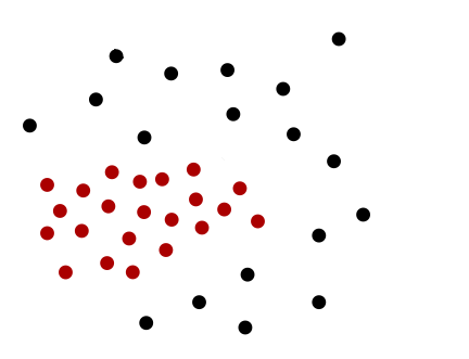
When hyperplanes are visualized, it is usually understood that one primarily cares about hyperplanes in higher-dimensional spaces where they are much more expressive, despite the illustration depicting an instance in $2$-d or $3$-d. But this time, think of the problem instance below in literal 2-d space:

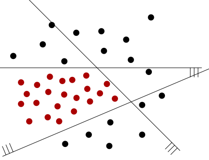
No hyperplane can classify this instance correctly, but consider a combination of these three hyperplanes:

By letting $h\left(p\right)={\sigma }_{\text{sign}}\left(h_1\right(p)+h_2(p)+h_3(p)-2.5)$ where $h_i$ is the predictor corresponding to the $i$-th hyperplane and ${\sigma }_{\text{sign}}$ is the sign function, we have constructed a predictor $h$ which has zero empirical error on this training instance.

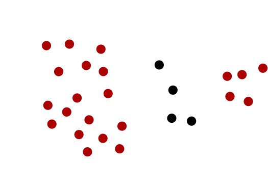
Perhaps more surprisingly, this trick can also learn non-convex areas. The instance below,

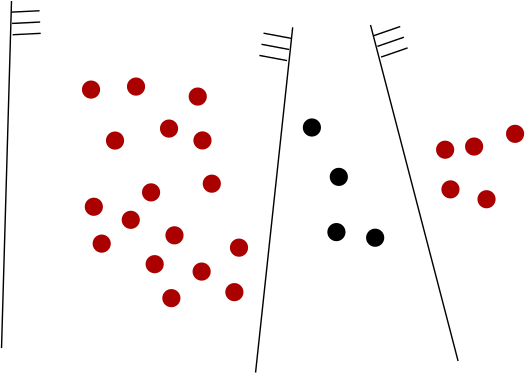
will be classified correctly by letting $h\left(p\right)={\sigma }_{\text{sign}}\left(h_1\right(p)+2h_2(p)+2h_3(p\left)\right)$, with the $h_i$ (ordered left to right) defined like so:

These two examples illustrate that the resulting class is quite expressive. The question is, how to learn such a linear combination?

II

First, note that hyperplanes are just an example; the framework is formulated in terms of a learning algorithm that has access to a weak learner, where

An algorithm $A$ is called a $\gamma$-weak learner for a hypothesis class $H$ iff there is a function $w^{\ast }:(0,1)\to N$ such that, for any probability distribution $D$ over $X\times Y$ and any failure probability $\delta \in (0,1)$, if $S$ consists of at least $w^{\ast }\left(\delta \right)$ i.i.d. points sampled via $D$, then with probability at least $1-\delta$ over the choice of $S$, it holds that $\ell \left(A\right(S\left)\right)\le \frac{1}{2}-\gamma$.

If you recall the definition of PAC learnability back from chapter 1 [LW · GW], you'll notice that this is very similar. The only difference is in the error: PAC learning demands that it be arbitrarily close to the best possible error, while a weak learner merely has to bound it away from $\frac{1}{2}$ by some fixed amount $\gamma$, which can be quite small. Thus, a weak learner is simply an algorithm that puts out a predictor that performs a little bit better than random. In the first example, the upper hyperplane could be the output of a weak learner. The term "boosting" refers to the process of upgrading this one weak learner into a better one, precisely by applying it over and over again under the supervision of a smartly designed algorithm –

– which brings us back to the question of how to define such an algorithm. The second example (the non-convex one) illustrates a key insight here: repeatedly querying the weak learner on the unaltered training instance is unlikely to be fruitful, because the third hyperplane by itself performs worse than random, and will thus not be output by a $\gamma$-weak learner (not for any $\gamma \in R_{+}$). To remedy this, we somehow need to prioritize the points we're currently getting wrong. Suppose we begin with the first two hyperplanes. At this point, we have classified the left and middle cluster correctly. If we then weigh the right cluster sufficiently more strongly than the other two, eventually, $h_3$ will perform better than random. Alas, we wish to adapt our weighting of training points dynamically, and we can do this in terms of a probability distribution over the training sequence.

Now the roadmap for defining the algorithm which learns a predictor on a binary classification problem via boosting is as follows:

• Have access to a training sequence $S$ and a $\gamma$-weak learner $A_{\gamma }$
• Manage a list of weak predictors which $A_{\gamma }$ has output in previous rounds
• At every step, hand $A_{\gamma }$ the training sequence $S$ along with some distribution $D^{\left(t\right)}$ over $S$, and have it output a $\gamma$-weak predictor $h_{t+1}$ on the problem $(S,D^{\left(t\right)})$, where each point in $S$ is taken into account proportional to its probability mass.
• Stop at some point and output a linear combination of the $h_i$

The particular algorithm we will construct is called Ada-Boost, where "Ada" doesn't have any relation to the programming language, but simply means "adaptive".

III

Let's first look into how to define our probability distribution, which will be the most complicated part of the algorithm. Suppose we have our current distribution $D^{\left(t\right)}$ based on past predictors $h_1,...,h_{t-1}$ output by $A_{\gamma }$, and suppose further that we have computed weights $w_1,...,w_{t-1}$ such that $w_i$ measures the quality of $h_i$ (higher is better). Now we receive a new predictor $h_t$ with quality $w_t$. Then we can define a new probability distribution $D^{(t+1)}$ by letting

$D^{(t+1)}\left(\right(x_i,y_i\left)\right)\propto D^{\left(t\right)}\left(\right(x_i,y_i\left)\right)\cdot e^{-w_t{y}_i{h}_t\left(x_i\right)}\forall i\in \left[m\right]$

where we write $\propto$ rather than $=$ because the term isn't normalized; it will equal the above scaled such that all probabilities sum to 1.

The term $y_i{h}_t\left(x_i\right)$ is $1$ iff predictor $h_t$ classified $x_i$ correctly. Thus, the right component of the product equals $e^{-w_t}$ iff the point was classified correctly, and $e^{w_t}$ if it wasn't. If $h_t$ is a bad predictor and $w_t$ is small, say ${10}^{-3}$, the two terms are both close to 1, and we don't end up changing our weight on $(x_i,y_i)$ very much. But if $h_t$ is good and $w_t$ is large, the old weight $D^{\left(t\right)}\left(\right(x_i,y_i\left)\right)$ will be scaled significantly upward (if it got the point wrong) or downward (if it got the point right). In our second example, the middle hyperplane performs quite well on the uniform distribution, so $w_2$ should be reasonably high, which will cause the probability mass on the right cluster to increase and on the two other clusters to decrease. If this is enough to make the right cluster dominate the computation, then the weak learner might output the right hyperplane next. If not, it might output the second hyperplane again. Eventually, the weights will have shifted enough for the third hyperplane to become feasible.

IV

Now let's look at the weights. Let ${ϵ}_t={\ell }_S^{0-1}\left(h_t\right)$ be the usual empirical error of $h_t$, i.e., ${ϵ}_t=\frac{1}{m}|\left\{\right(x,y)\in S|h_t(x)\ne y\}|$. We would like $w_i$ to be a real number, which starts close to $0$ for ${ϵ}_t$ close to $\frac{1}{2}$ and grow indefinitely for ${ϵ}_t$ close to 0. One possible choice is $w_t:=\frac{1}{2}\ln (\frac{1}{{ϵ}_t}-1)$. You can verify that it has these properties – in particular, recall that $h_t$ is output by a weak learner so that its error is bounded away from $\frac{1}{2}$ by at least $\gamma$. Because of this, $\frac{1}{{ϵ}_t}$ is larger than $2$ so that $\frac{1}{{ϵ}_t}-1$ is larger than $1$ and $w_t$ is larger than $0$.

V

To summarize,

AdaBoost ($A_{\gamma }$ : weak learner, $S$ : training sequence, $T:N_{+}$)

$D^{\left(0\right)}\leftarrow (\frac{1}{m}\cdots \frac{1}{m})$

for $(t\leftarrow 1\text{to}T)$ do

$h_t\leftarrow A_{\gamma }(S,D^{(t-1)})$

${ϵ}_t\leftarrow \frac{1}{m}|\left\{\right(x,y)\in S|h_t(x)\ne y\}|$

$w_t\leftarrow \frac{1}{2}\ln (\frac{1}{{ϵ}_t}-1)$

$D^{\left(t\right)}\leftarrow \text{normalize}((D_i\cdot e^{-w_t{y}_i{h}_t\left(x_i\right)}{)}_{i\in \left[m\right]})$

endfor

return $f:x\mapsto {\sigma }_{\text{sign}}\left({\sum }_{t=1}^T{w}_t{h}_t\right(x\left)\right)$

end

VI

If one assumes that $A_{\gamma }$ always returns a predictor with error at most $\frac{1}{2}-\gamma$ (recall that it may fail with probability $\delta$), one can derive a bound on the error of the output predictor. Fortunately, the dependence of the sample complexity on $\delta$ is only logarithmic, so $\delta$ can probably be pushed low enough that $A_{\gamma }$ is unlikely to fail even if it is called $T$ times.

Now the error bound one can derive is $e^{-2{\gamma }^{2}T}$. Looking at this, it has exactly the properties one would expect: a higher $\gamma$ pushes the error down, and so do more rounds of the algorithm. On the other hand, doing more rounds increases the chance of overfitting to random quirks in the training data. Thus, the parameter $T$ allows one to balance the overfitting vs. underfitting tradeoff, which is another nice thing about AdaBoost.The book mentions that Boosting has been successfully applied to the task of classifying gray-scale images into 'contains a human face' and 'doesn't contain a human face'. This implies that human faces can be recognized using a set of quantitative rules – but, importantly, rules which have been generated by an algorithm rather than constructed by hand. (In that case, the weak learner did not return hyperplanes, but simple predictors of another form.) In this case, the result fits with my intuition (that face recognition is the kind of task where a set-of-rules approach will work). It would be interesting to know how well boosting performs on other problems.

1 comments

Comments sorted by top scores.