"Newton's laws" of finance

post by pchvykov · 2024-06-21T09:41:21.931Z · LW · GW · 3 comments

Contents

  Geometric Brownian Motion
  Ergodicity Economics and rational choices
  Clarifying confusions
  Practical consequences
  Cooperation and insurance
None
3 comments

[NOT financial advice! In fact I'll really be showing some generic math here – and it's up to you if you apply it to investments in stocks, projects, relationships, ideas, skills, etc.] 

As I’ve been thinking about some economic theories and working on a personal investment algorithm, I kept coming across ideas that seemed entirely fundamental to how one should think about investing – and yet I could not find any reasonable references that would give a clear overview of these. Thus it took me some time of playing with algorithms and math to figure out how it all fits together – and now seems perfectly obvious. But just as it was not obvious to me before, I now have conversations with friends who also get confused. I suspect this comes from investment being taught from a “wrong” starting points – so people have a different idea of what is “basic” and what is “advanced.”

Two caveats I have to mention here: First, I’m a physicist, and so my idea of what is “basic” is entirely informed by my background. I do suspect this stuff might seem more “advanced” to someone not as comfortable with the math I’ll be using. By the same token, this is probably why the typical “finance basics” seem very confusing and convoluted to me. Second, I’m a fan of Ergodicity Economics, and this post will be informed by their perspective. This perspective, while seems entirely correct to me, is not part of the “economics cannon” – and so may be contested by some. Still, I think the math I will show and the conclusions relevant to investing are generally correct and accepted as such (just a bit hard to find). 

Geometric Brownian Motion

The starting point for everything I'm going to say is the assumption that investments follow Geometric Brownian Motion (GBM) dynamics:

$${\partial }_{t}x=x\cdot (\mu +\sigma \xi )\left[1\right]$$

where $x$ is your wealth (e.g., stock price, or project value),  $(\mu ,\sigma )$ are parameters characterizing the investment (return and volatility respectively), and $\xi \left(t\right)$ is standard uncorrelated white Gaussian noise process (so that $⟨\xi \left(t\right)⟩=0$ and $⟨\xi \left(t\right),\xi \left(t^{\prime }\right)⟩=\delta (t-t^{\prime })$, where $⟨\cdot ⟩$ denotes average over noise realizations, and, for experts, we take Itô noise). This model is at the core of much of quantitative finance, as it captures both the random fluctuations and compounding growth of the investment. It is also a model that researchers "love to hate," as it is oversimplified in many aspects. Just to list a few problems with it:

1. Real stock price fluctuations have a heavy-tail distribution, meaning that large fluctuations are much more likely than the Gaussian noise would predict – and such rare events are core to long-term price changes
2. Price fluctuations are correlated over time – unlike the "white noise" assumption here
3. The assumption that $(\mu ,\sigma )$ parameters are constant is unrealistic, and estimating them locally from historical data is not obvious – especially when you have many stocks and need to get the matrix of cross-correlations ${\sigma }_{ij}$.

Nonetheless, just as in physics we research the failure points of classical mechanics, so here these violations of the GBM model are "exceptions that prove the rule." Realistically, the jury is still out on whether this is a good starting point for quantitative finance models, but at least for this post, we will run with it and see what we get. The benefits of this model is that it's simple enough to allow analytical calculations, seems to capture a large part of financial behaviors, and is rich enough to allow for some interesting counter-intuitive conclusions and predictions. I think thinking of it as "Newton's law of finance" wouldn't be entirely wrong. 

First, let's consider the basic GBM dynamics and immediate consequences of this model. We notice that by averaging over noise realizations in eq.[1], we get

$${\partial }_t⟨x⟩=\mu ⟨x⟩\Rightarrow ⟨x⟩\propto e^{\mu t}\left[2\right]$$

If we numerically simulate 100 GBM trajectories (gray) and plot their mean (blue), median (red), and the above prediction (dotted black), we get (note the log scale):

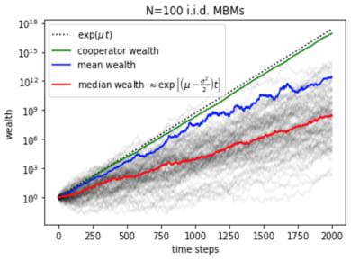
This clearly shows that the above prediction is systematically higher than the actual numerical performances. Even the numerical mean (blue) only somewhat tracks with this prediction for the first 1000 time-steps, before becoming hopelessly wrong. This discrepancy, coming from little-known weirdness of stochastic calculus, will be the core of the counterintuitive behaviors we will see in the rest of the post. 

The issues comes because the price distribution resulting from GBM has a heavy-tail (is log-normal to be precise), and thus for any finite number of trajectories, the ensemble average will be very sensitive to how well you sample the tail – and so sensitive to outliers. In fact, if instead of 100, we simulated 1000 trajectories in the above plot, the ensemble mean (blue) would track with the prediction only a bit longer (to 1500 steps – scaling as log of ensemble size). Either way, the prediction in eq.[2] breaks down for any finite number of samples – and so in any practical application. We can take this as a cautionary tale about relying too much on averages in general!

The median (red), on the other hand, is much more representative of what the actual prices are doing. We can also analytically get its behavior by changing variables:

$${\partial }_t\log x=(\mu -\frac{{\sigma }^2}{2})+\xi \Rightarrow ⟨\log x⟩=(\mu -\frac{{\sigma }^2}{2})t+const\left[3\right]$$

This shows that in log-space, the process is a simple Brownian motion process, and thus has a steady linear drift (as we also see in figure 1 above). However, the drift rate is not $\mu$as we might have expected, but is reduced by a "volatility drag." This drag comes from a technical point in stochastic calculus, Itô's lemma (coming from the non-differentiability of the white noise process $\xi \left(t\right)$). This way, we see that the correct growth exponent to understand GBM process is given by the "geometric growth rate" $g=\mu -\frac{{\sigma }^2}{2}$. 

Ergodicity Economics and rational choices

Since this volatility drag will be core to the rest of our results, let's understand it from another angle. GBM process in eq.[1] is non-ergodic, meaning that our ensemble average over noise realizations is not the same as the time-average over a given trajectory (as we saw above). This may seem like a technical point, but it actually has profound implications for what is "optimal" or "rational" behavior for a given agent. When thinking about whether or not to take a given bet (or investment), we are typically taught that the right choice is the one that gives us maximal expected return (implying expectation over random noise). The implicit assumption there is that if we repeat that same thinking many times, this will also give us the best long-term outcomes. But this logic breaks down when our bets across time are not independent of each other, as is the case when we have compound growth. There, we need to consider the impact of our bet not just on our immediate wealth, but also on the future games / investments we can make – on the doors it opens or closes. 

One simple illustration of this is in the following game (cf. St. Petersburg paradox): you have a 50-50 chance of either tripling your wealth, or losing it all – do you play? The expected returns of playing are positive at every turn, but if you keep playing each time, you are guaranteed to lose everything. 

Since for GBM, we saw that $\log x$ undergoes simple Brownian motion (no compounding), it is thus ergodic, and so the noise-average here does tell us also about long-term performance – see eq. [3]. In practice, this means that our GBM analysis above shows that the rational long-term strategy is to maximize geometric growth rate $g$, which will be the time-averaged growth rate for any noise realization (see fig.1). As an exercise, you can check that $g$ for the above game is <0 – correctly predicting the loss.

Clarifying confusions

This is a good point to pause and clarify some confusions I see in the basic finance readings. 

Simple returns $r\left(t\right)=\frac{x(t+1)-x\left(t\right)}{x\left(t\right)}$ and log returns $r_l\left(t\right)=\log \frac{x(t+1)}{x\left(t\right)}$ are not interchangeable. 
I see people discussing them as if the choice to use one or the other is a matter of convenience or application – but these are just different quantities! The confusion comes because these can be shown to be equivalent at first-order in Taylor expansion (for slow variation $\dot{x}=dx/dt$): 
$r_l\left(t\right)=\log \frac{x\left(t\right)+\dot{x}\left(t\right)+\ddot{x}\left(t\right)/2+...}{x\left(t\right)}\approx \log (1+\frac{\dot{x}\left(t\right)}{x\left(t\right)})\approx \frac{\dot{x}\left(t\right)}{x\left(t\right)}\approx r\left(t\right)$. 
However, from the above analysis, we clearly see that for GBM $⟨r\left(t\right)⟩=\mu$ and $⟨r_l\left(t\right)⟩=\mu -\frac{{\sigma }^2}{2}$, and so the two will give clearly different values and cannot be compared. The above Taylor-expansion argument is wrong because for GBM $\ddot{x}\left(t\right)$ is formally divergent, and so cannot be dropped. 

Sharpe ratio $Sa=\frac{\mu }{\sigma }$ is not informative of investment growth. 
This is the most common metric used to evaluate stocks or investment portfolios in finance. At first glance it seems reasonable – it's just the signal-to-noise ratio for our returns. However, this only tells us about our performance for one given time-step, and it ignores the effects of compounding growth over time. The compounding long-term growth rate is instead captured by $g=\mu -\frac{{\sigma }^2}{2}$, as we saw.
We can see this problem already from dimensional analysis. From GBM eq.[1], we see that $\mu$ has units of $[time{]}^{-1}$ and $\sigma \sim [time{]}^{-1/2}$ (because $\xi \sim [time{]}^{1/2}$). This means that $g\sim [time{]}^{-1}$, which is what we expect for a growth rate. Sharpe ratio, however, has $Sa\sim [time{]}^{-1/2}$, which means that we have to explicitly specify the timescale at which $Sa$ is given, and to go from, e.g., daily to annual $Sa$, we need to multiply by $\sqrt{365}$, which is awkward. 

In practice, what $Sa$ does tell us is our chances of losing money on the given timescale – since it basically tells us how many sigmas our expected wealth will be from 0. In my opinion, this isn't the most informative piece of information when choosing an investment, since it tells us nothing about expected growth.

To get a bit more real-world grounding to all this abstract theory, we can look at the values of the $(\mu ,\sigma )$ parameters for real-world stock data. Getting the price data from Yahoo finance for about 2000 NASDAQ stocks, we can calculate the mean and variance of simple daily returns, and then show them on a scatter plot (so each point here is one stock):

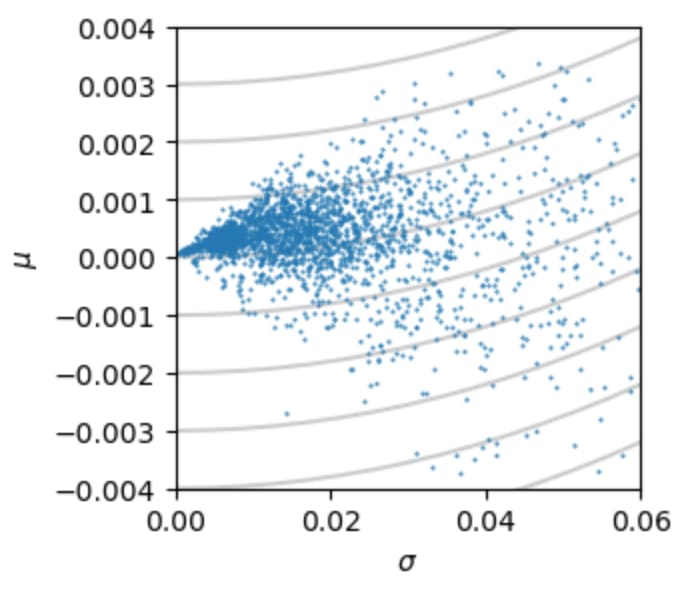
We immediately notice the characteristic conus shape of this distribution – known as the Markowitz bullet. It is bounded by an "efficient frontier," beyond which no stock can give a higher return for a given level of risk. We can see that the efficient frontier is nearly straight – meaning it's given by some maximal Sharpe ratio  $Sa=\frac{\mu }{\sigma }=const$. The reasons for this may be fundamental, or may be because $Sa$ is used so much in finance that the trading dynamics regulate stocks from going much above the typical $Sa$maximum (which is around 0.1 daily Sharpe $\approx 2$ annual Sharpe). Note that on the bottom we have a similar efficient frontier – which is equally necessary because we can make money shorting stocks that reliably drop. 

The gray parabolas in fig.2 above are lines of constant $g=\mu -\frac{{\sigma }^2}{2}$, which suggest that investing in the high-risk high-reward stocks in the upper right corner of this distribution should give the highest time-averaged growth rate. The issue with that strategy in practice comes from the problems with the original assumptions of the GBM model – we're never sure if the $(\mu ,\sigma )$ we got historically will hold going forward, and we're typically going to have more volatility than we expect due to the non-Gaussian heavy tails. 

Practical consequences

So what does all this setup practically tell us about the world? One immediate consequence of the expression for $g=\mu -\frac{{\sigma }^2}{2}$ is that volatility directly reduces our returns. This cleanly shows the benefit of portfolio diversification – if we can reduce the noise by averaging over fluctuations of many different assets, then we can increase our time-average returns. Interestingly, however, this will only work if we rebalance regularly. Let's see why. 

To start, consider that we have $N$ different stocks, each with the same $(\mu ,\sigma )$. Assuming their price follows GBM, we are again in the scenario of fig.1 above. If we simply buy and hold all these assets at equal proportions, then our portfolio will grow as their mean – following the blue line (fig.1). We see that eventually this will grow at the same rate as each individual stock $\mu -\frac{{\sigma }^2}{2}$, and so while it might seem like an improvement early on, we haven't gained much in the long run. This is because over that initial period, as the prices diverge, we get only a few stocks dominating our portfolio, and so we lose the benefits of diversification. In the opposite extreme, if we rebalance our portfolio every single day to keep exactly equal allocation of wealth to each stock, then we directly average out the noise across stocks, thus reducing the portfolio volatility to $\frac{\sigma }{\sqrt{N}}$ (by the central limit theorem), and so making portfolio growth rate $g=\mu -\frac{{\sigma }^2}{2N}$. The resulting stochastic process is the green line in fig.1 – and shows nearly deterministic growth much above that of individual stocks. In practice, due to trading fees and the bid-ask spread, we need not rebalance daily, but instead only when portfolio mean growth rate starts dropping – so in fig.1, each ~200 time-steps. 

When $(\mu ,\sigma )$ are different for different stocks (as in fig.2), we can find the optimal allocations of our portfolio according to Kelly portfolio theory. All this means is maximizing the geometric growth rate, which for a portfolio of allocation fractions $f_i$ takes the form $g={\sum }_i{\mu }_i{f}_i-\frac{1}{2}{\sum }_{ij}{\sigma }_{ij}{f}_i{f}_j$. Note that ${\sigma }_{ij}$ here is the covariance matrix for stock returns (also accounting for cross-correlations), with $\{i,j\}$ indexing the different stocks. This expression for $g$ again assumes regular (e.g., daily) rebalancing. 

But before you invest all your money into this scheme though, a few warnings (I actually tried to develop a trading algorithm based on this, and was, of course, disappointed – but I learned a lot). First, all of this is pretty standard knowledge in quantitative finance, and so there is little reason to believe this effect hasn't yet been arbitraged away (such rebalancing will tend to correlate stock prices, reducing available gains). Although I'm still surprised that this isn't more standard – for example, I'm not sure why we still have portfolios that don't rebalance, like Dow Jones (which is allocated according to asset price). Second, when we have correlations among stocks, so that ${\sigma }_{ij}$ is non-diagonal, it becomes much harder to significantly reduce our volatility through diversification. I was surprised how strong this effect is – even small correlations drastically drop the value of diversifying. To make matters worse, it is very difficult to accurately estimate the full matrix ${\sigma }_{ij}$ from data. And finally, once again, I have to refer to the limitations of the GBM modeling assumptions.

Cooperation and insurance

In Ergodicity Economics, this regular "rebalancing" step that leads to improved collective performance is used to argue for the selfish benefit of cooperation – where we pool and share our resources on a regular basis [see here]. This may seem counterintuitive at first – how could reshuffling wealth in this way make the overall economy grow faster? But again, this is explained by the dependence of bets across time in the context of compound growth, so we cannot treat individual investments as isolated events. 

A parallel argument can then be made to explain the value of buying insurance – simultaneously for the insurer and for the insured. To give some intuition for this, in a compound-growth environment, what ultimately matters is not absolute wealth, but fractional wealth (you live on log-scales). This way, the less wealth you have, the more certain risks "cost" you in the long-run. This allows for insurance-premium prices that end up being a win-win for both parties in the long run [see here]. 

---

To conclude, I think this GBM setup is a really pretty piece of math, whose simplicity suggests that it might be a good minimal model for many aspects of the world beyond just finance. Whenever we invest our time, resources, intelligence, or emotions into something that has some "compounding growth" property, we can take inspiration from this model. One big takeaway for me is to remember that in those contexts, it is wrong to optimize expected returns for an individual game – and instead we need to look at the compounding long-term ripples of our strategy. So rather than seeing my decisions in isolation, I see each one as a "practice" that builds a habit. Ergodicity Economics suggest that this realization and its integration into our decisions and policy may be key to building a more sustainable world. But for this to work, we must implemented these insights not only collectively, but also individually. So, mind the volatility drag, and remember to (re)balance!

[Cross-posted from my blog pchvykov.com/blog]

3 comments

Comments sorted by top scores.