Addendum: basic facts about language models during training

post by beren · 2023-03-06T19:24:45.246Z · LW · GW · 2 comments

Contents

  Weight distribution
  Similarity with non-deduplicated models
    Non-deduped
    Deduped
None
2 comments

This post is a follow-up to our previous work [LW · GW] on language model internals through training based on great additional suggestions by commenters. If you haven’t read the original post, please read it first. This post is part of the work done at Conjecture. 

Our previous post created a lot of very helpful discussion and suggestions for further experiments by commenters. Especially interesting was the discussion of what exactly was the final weight distribution that the model evolved towards is, and whether this distribution could be directly sampled from to serve as an initialization for future models. While we do not have a straightforward parametric form for such a distribution, we have made some further progress on this question, and now believe that the final distribution is close to the one expected by naively computing the sums and products of Gaussian distributions that would characterize the residual stream at initialization. 

Weight distribution

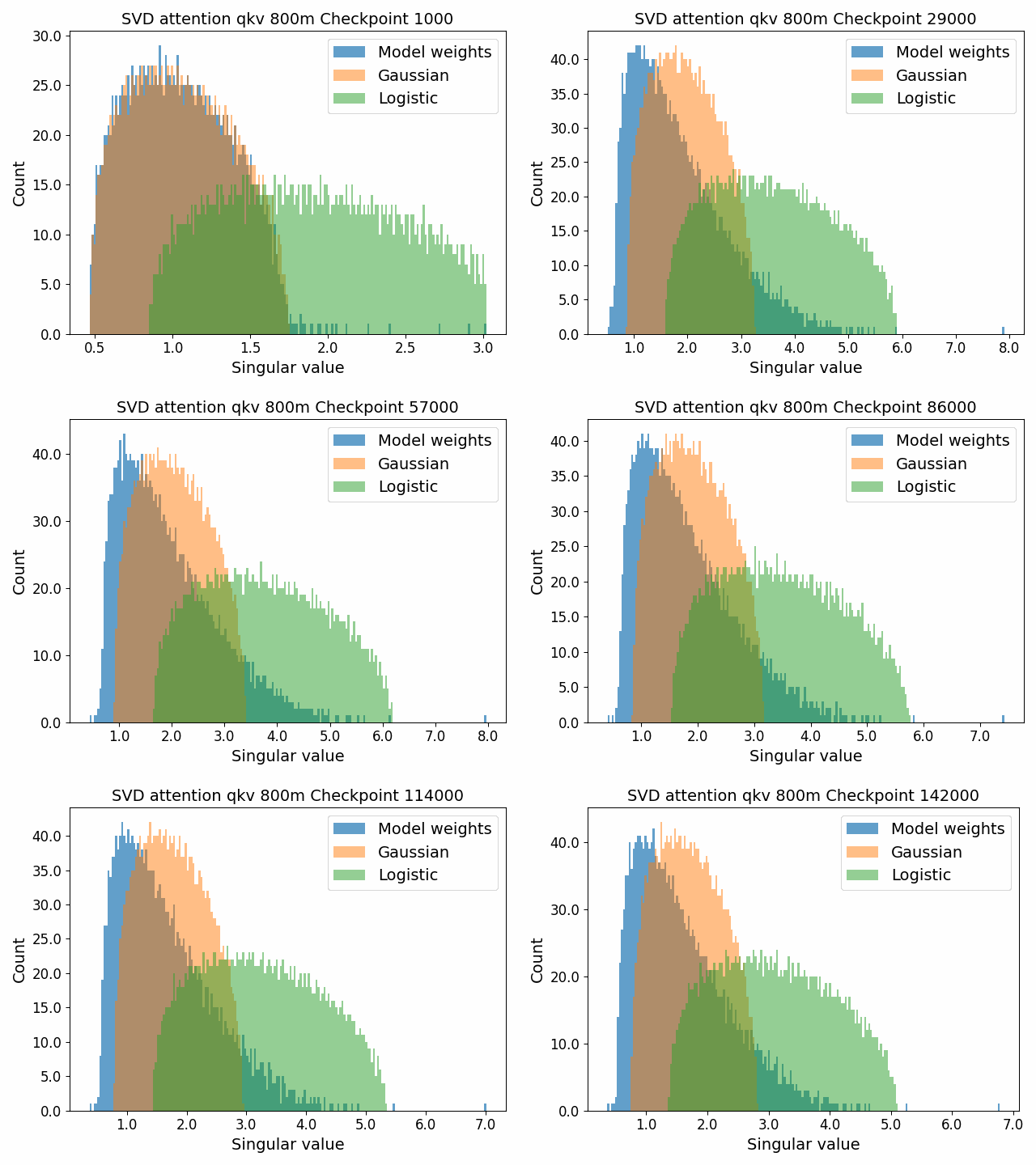
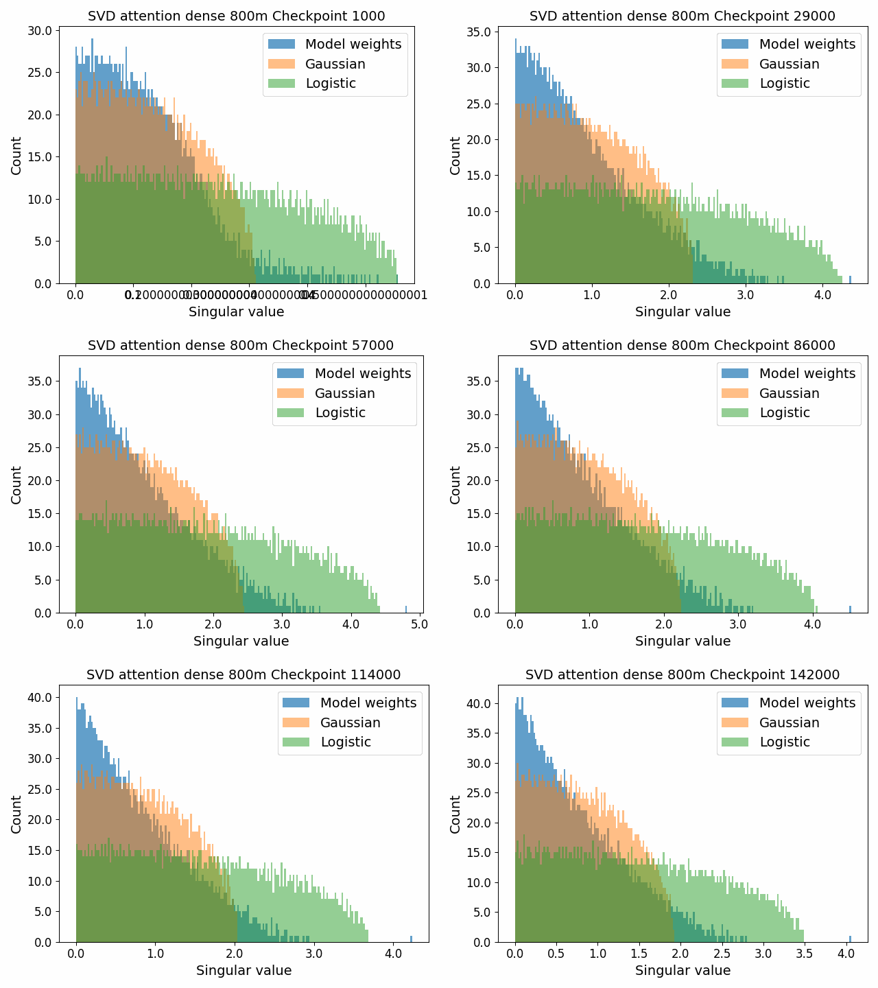
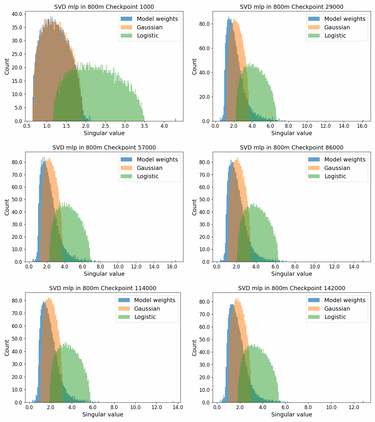
To begin, we showcase a new approach to visualizing the nature of the weight distributions through training: animation of the histogram of the singular values compared to other distributions such as the Gaussian and Logistic distributions. Below we show animations of these distributions for the attention QKV and output matrices as well as the MLP input and output matrices for the 800m model. For these animations we choose the weight block approximately in the middle of the network – i.e. block = length // 2.  Similar distributions were observed in all the other pythia model sizes (up to 1.3b). For comparison we also show the singular value histograms for equivalent Gaussian and logistic distributions. The Gaussian and logistic distribution histograms were plotted by fitting the parameters of Gaussian or Logistic distributions to the weight distribution, then sampling a tensor of the same shape as the weight matrix, then performing an SVD on that tensor to obtain the singular values.

 

What we typically observe forming is a highly consistent but unusual distribution which both has a much higher concentration of zero singular values than even a Gaussian, reflecting sparsity or a large number of extremely small directions, as well as an extremely long tail which is much heavier than either logistic or power-law distributions. This distribution is highly consistent and appears to form for most of the weight distributions in the model as shown above, where the pattern is most apparent in the attention QKV and the MLP weight matrices while the output attention matrix is much more Gaussian, although it still displays a small heavy tail. Even more interestingly, it is apparent that this special weight distribution forms rapidly at the beginning of training and then is largely consistent throughout.
 

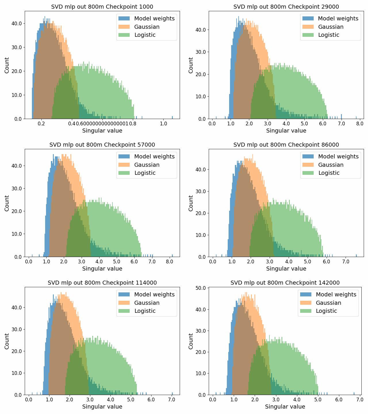
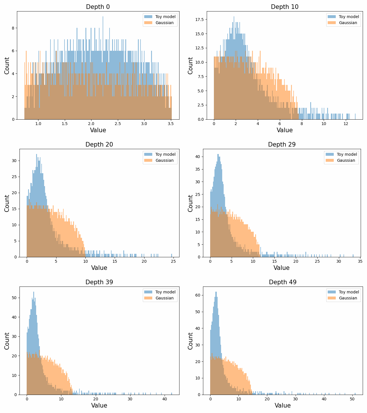
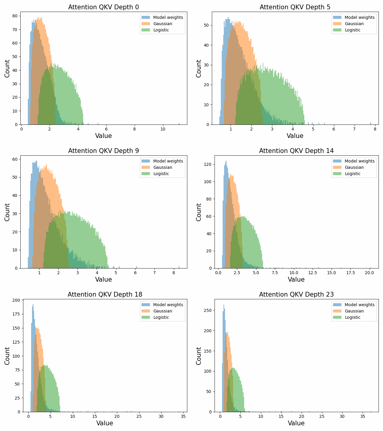
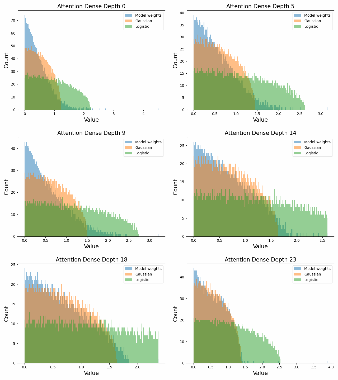
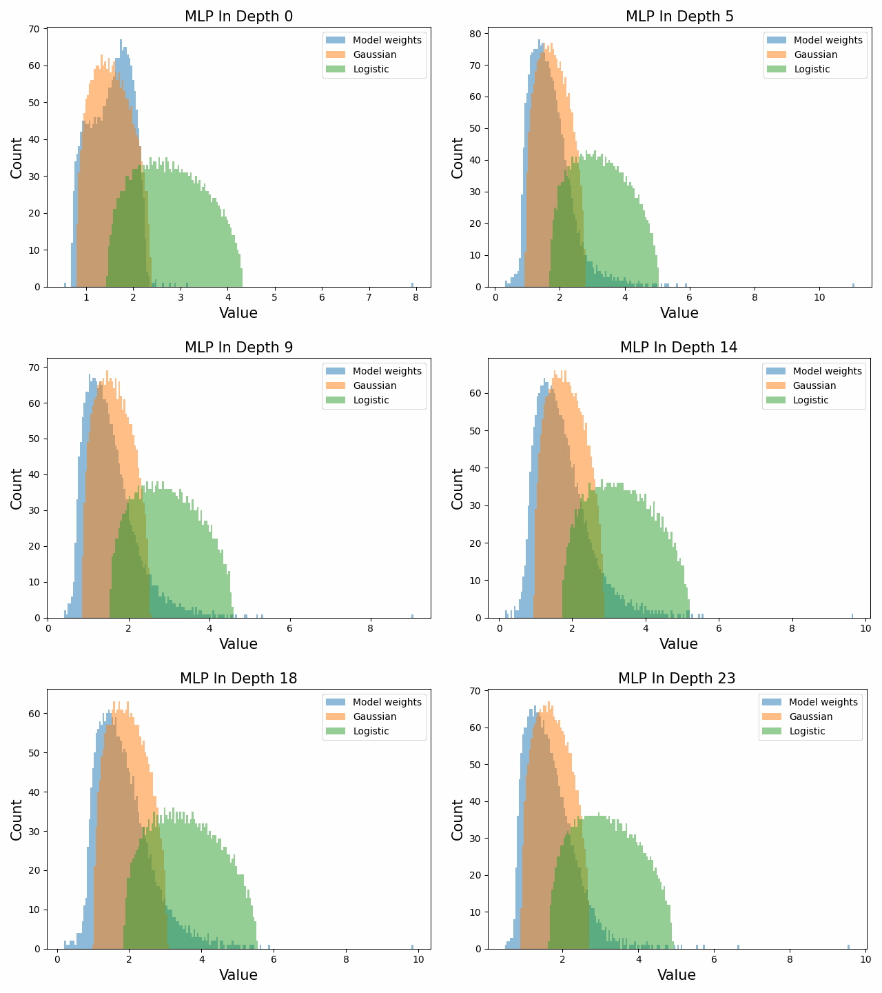
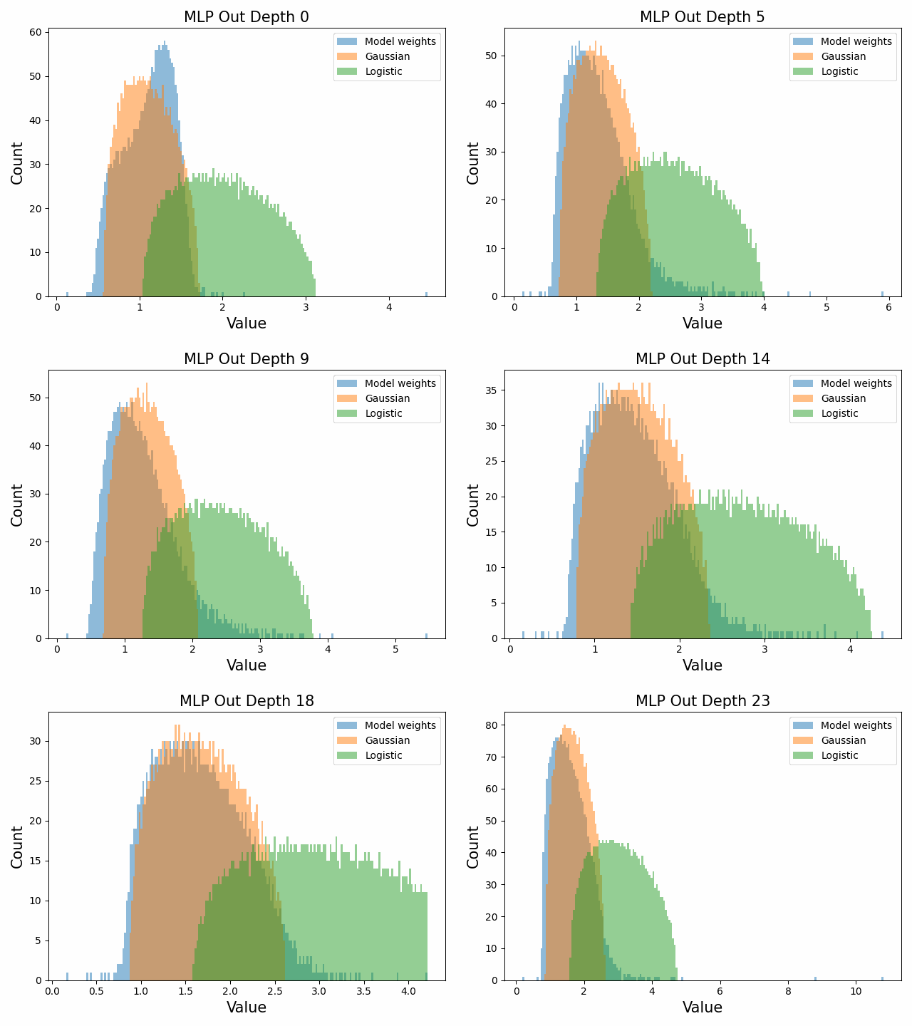
However, we were able to find a distribution which approximately and qualitatively matched the behaviour we observed – namely the distribution you get by simulating the evolution of activations through the residual stream with Gaussian weights. This distribution becomes non-gaussian because the distribution of the product of Gaussian random variables is not Gaussian (even though the joint distribution of multiple independent Gaussians is Gaussian). If we consider the set of all possible paths through a residual network, we observe that there are a large number of ‘product paths’ through the network (in fact the paths are identical to the polynomial expansion $(1+x{)}^D$ ). This is obvious if we imagine a two layer residual network with blocks $x_1$ and $x_2$. If we think of all possible paths, there is the direct path through the residual from input to output, the path through $x_1$ then up the residual to the output, the path up the residual to $x_2$, then to the output, and then the path through both $x_1$ and $x_2$. Assuming each block $x$ simply performs a multiplication by a random Gaussian matrix, we can then compute the distribution at the output of various depths. Clearly, this begins as Gaussian with a depth 1 residual network (sums of Gaussians are Gaussian) but then each product path of a depth greater than 1 adds a non-gaussianity into the sum. The output distribution of this process ends up looking qualitatively similar to the observed distributions of the weights, with certain differences. Below, we simulate a toy model with a residual stream dimension of $1024\times 1024$ and with a Gaussian critical initialization of $\frac{1}{\sqrt{\text{width}}}$, which is necessary to preserve the norms of the product contributions which would otherwise vanish or explode. 

We observe that qualitatively this distribution looks similar to our weight distribution, especially for middling depths –around 10-20 which is approximately the same as the 800m model’s true depth of 16. If this hypothesis is true, it may mean that the ideal weight distribution may be primarily shaped not by the dataset but by the natural inductive biases of the architecture which is reflected in the activation distribution at initialization. Moreover, by comparing the distribution of the model weights to the toy model at different depths, we may perhaps be able to estimate the ‘effective depth’ of the network. By effective depth, we mean the average depth of paths through the residual network that contribute most to the output distribution. Unlike in a hierarchical network such as a CNN, in a residual network this is not necessarily the actual depth of the network, since information from shorter paths can simply persist in the residual stream without being modified.  

Also of interest is the question of how the distribution of singular values changes with depth through the network. If our hypothesized generative process for the weight distribution is correct, it would predict that the distributions later in the network should be more Gaussian, since they have less depth (and hence non-gaussianity) to go before the network’s output. We test this hypothesis by plotting the evolution of the singular value histogram of the weight matrices of the 1.3B Pythia model with depth.

What we observe is that this approximately seems to hold true for the ‘output’ weight matrices (MLP out and attention dense) but not for the ‘input’ weight matrices, which instead appear either approximately stable or start developing even heavier tails towards the end of the network, for reasons that are unclear.

Similarity with non-deduplicated models

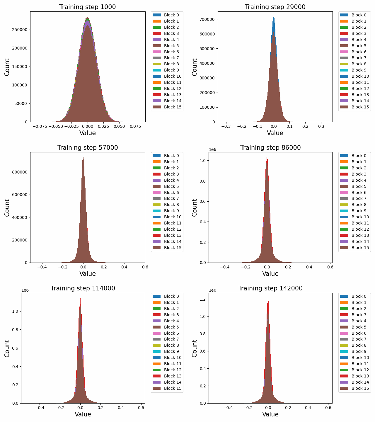
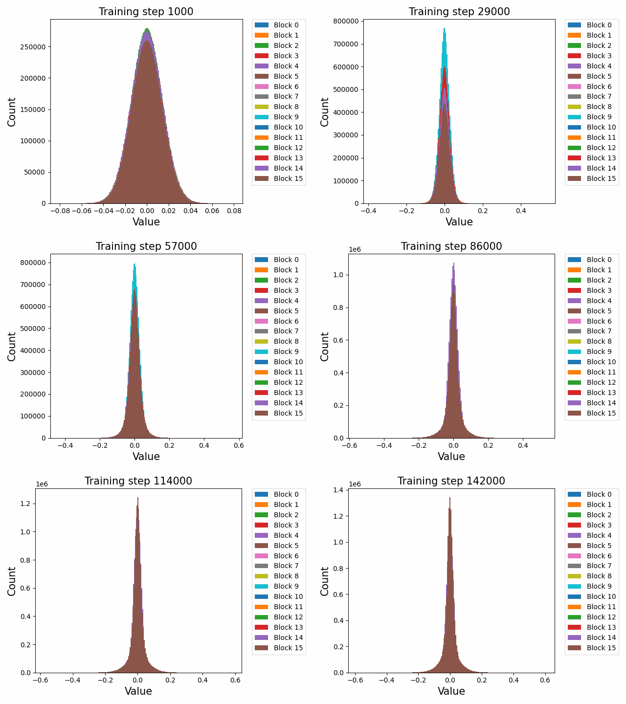
Finally, a comment by thomwolf [LW · GW] asked about how consistent our findings are across different model initializations, as exemplified by the difference between deduplicated and non-deduplicated models, since the deduplication is not expected to affect the model too much. By deduplication we mean whether the dataset has been strongly purged of duplicate documents (which may slightly mess up language model training) or not.  We plotted a number of weight statistics and histograms using the non-deduped models with the exact same methodology as the original deduped models. By eyeballing many of the graphs we observe that almost all of the same qualitative behaviours are identical between the two models, including the activation distribution histograms and the evolution of the weight norms during training (often including the block orderings). However, there are also some relatively minor discrepancies. For instance, we first show an animation of the evolution of the attention qkv weight matrices for the 800m model for both the deduped and non-deduped models.

Non-deduped

Deduped

Where we observe extremely similar macro-level distributional patterns between the weights in both cases, including the heavy-tailed distribution we wish to understand.

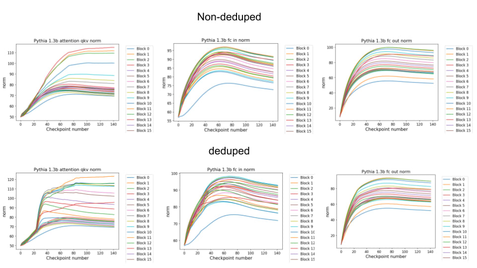
We observe a similar pattern if we do direct comparisons of the weight norms of the 1.3b model for the attention qkv and the MLP in and out matrices for both deduped and non-deduped models. Here again, we observe qualitatively extremely similar patterns between models especially in the MLPs where often even the timing and scale of the evolution of different blocks is extremely similar. We observe slightly more heterogeneity in the attention QKV weights where the deduped model appears to have a much sharper phase shift at checkpoint 20 than the non-deduped model, for reasons that are unclear. 

We have computed many more results along these lines than we can possibly show in this post. You can view all the plots directly in the associated repository which we have updated with this analysis.

Overall, we believe that our results demonstrate that our qualitative findings are almost always robust to this robustness implying that they are likely highly robust to different initializations of the same model architecture. The extent to which they are robust across architectures is largely unknown given that we do not have access to Pythia-like checkpoint suites for other architectures, and we think that this would be a highly fruitful avenue to pursue in future. In the case of language models, we are especially interested in the differences, if any, between standard GPT2 sequential transformer blocks vs the more parallel GPTJ blocks which Pythia used.

2 comments

Comments sorted by top scores.