Basic facts about language models during training

post by beren · 2023-02-21T11:46:12.256Z · LW · GW · 15 comments

Contents

  Weights show a rapid phase transition from Gaussian to extreme heavy tails
  So do residual stream and weight gradients
  Residual stream outliers grow rapidly then stabilize and decline
  MLP Weight norms rise, peak, and fall
  MLP biases increase and asymptote
  Layernorm weights and biases
  Euclidean Distance from initialization during training
  Analysis of de-embed and final layernorms 
  Tokenizer Embeddings are rapidly learnt then stabilize
  Power law weight spectra but differing behaviour across components
  Closeness to final SVD direction vectors grows exponentially and develops late
  Almost all of these effects are consistent across model scales
  Conclusion
None
15 comments

We thank Eric Winsor, Lee Sharkey, Dan Braun, Carlos Ramon Guevara, and Misha Wagner for helpful suggestions and comments on this post.

This post builds upon our last post [LW · GW] on basic facts about language model internals and was written as part of the work done at Conjecture. We will shortly release all plots and animations (only a very small subset made it into this post) as well as the code at this repository.

We are aware of there being some inconsistencies with the Pythia model suite due to different configs for different model sizes affecting the learning rate schedule. From discussions with the Pythia team, it appears unlikely that these materially affect the findings in this article. However, the nomenclature for the number of parameters in each model has since been updated in the Pythia docs. What we refer to as 19M is now 70M, 125M ->160M, 350M -> 410M, 800M -> 1B, and 1.3B -> 1.4B.
 

In this post, we continue the work done in our last post [LW · GW] on language model internals but this time we analyze the same phenomena occurring during training. This is extremely important in understanding how language model training works at a macro-scale and sheds light into potentially new behaviours or specific important phase transitions that may occur during training which deserve further study, as well as giving insight into the origin of phenomena that we consistently observe in fully trained models.

Throughout, as in the previous post, we do not delve into the details of specific circuits, but instead aim to provide a holistic macro-level view of the basic distributional properties of the LLM’s weights, activations, and gradients across training checkpoints. Although seemingly basic, we are not aware of any similar analysis having been performed publicly, and we believe that understanding these distributional phenomena seems generally important in constraining circuit-level theorizing as well as provides empirical links to the theoretical constructs such as the neural tangent kernel and tensor programs that can prove facts about specific limits. 

To perform our analysis, we use the open source Pythia model suite which contains a large number of checkpoints during training and was trained by EleutherAI and aims to use interpretability analysis to understand how representations develop across training. We agree with this goal and are happy to share our own analysis code etc.  The Pythia project trains models of different sizes on exactly the same data in exactly the same order so as to be able to understand how and when certain representations form both during training and across different model scales. The Pythia models we utilize range from 19M parameters to 1.3B. Each Pythia model has 142 checkpoints of stored weights, equally spaced every 1000 steps, which we sweep across to perform our analysis.

Weights show a rapid phase transition from Gaussian to extreme heavy tails

It was very helpfully pointed out in a comment on our previous post that the weight statistics were actually sharper and more heavy tailed than Gaussian. This is correct and we also found this when we fit histograms to logistics vs Gaussian distributions. Overall, we find that the activation distributions of GPT2 models are generally not Gaussian but somewhere in between the logistic $e^{-x}$ and the Gaussian $e^{-x^2}$, which indicates both heavier tails and a thinner bulk. This is extremely interesting since it means that the weight statistics must move away from their Gaussian initialization which implies a highly significant perturbation away from their original position. This is perhaps in contrast with some theories, such as NTK theory, which argue that for large models we should not expect the weights to diverge too much from their initial position.
 

The Pythia models provide us some insight into this since we can directly plot and animate the distribution of weights during training. We have shown some illustrative examples below. For the full suite of animations please see the associated GitHub.

Here we have animated the evolution of the attention QKV weights during training,

 

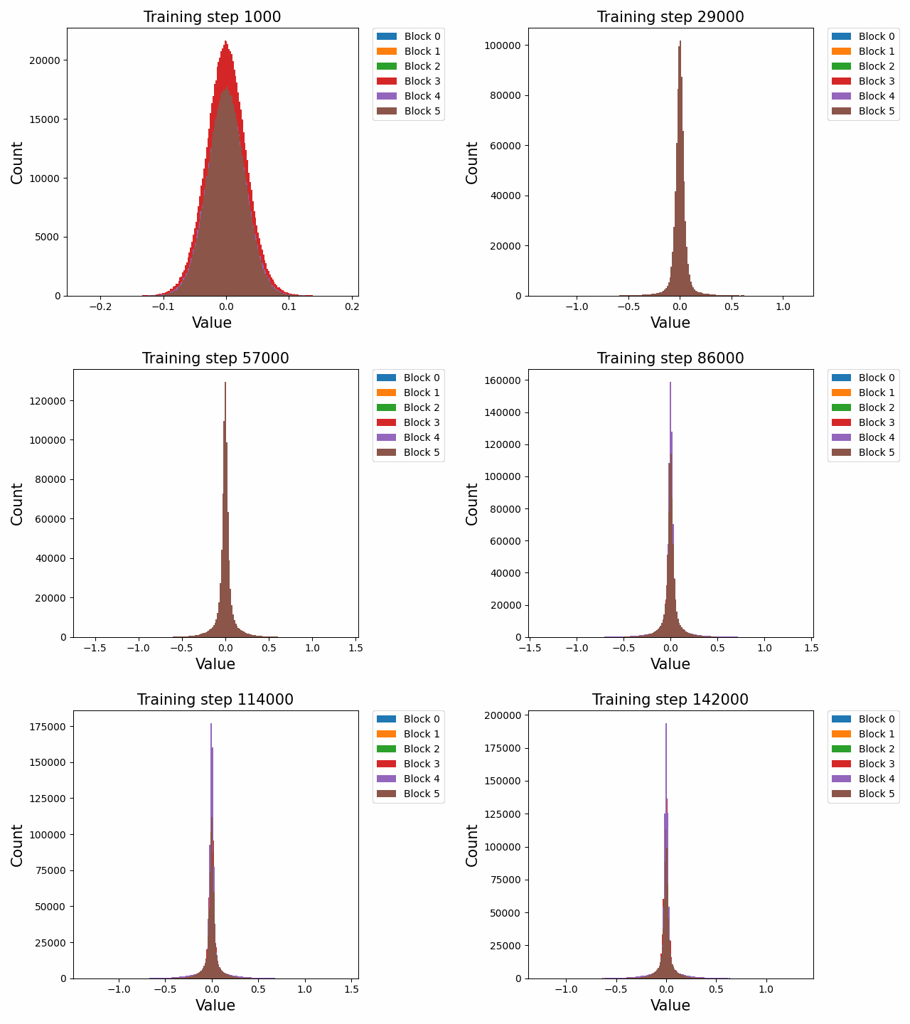
Of note is the relatively sudden shift to the logistic distribution which occurs relatively early on in training at about 20,000 out of 140,000 steps. This occurred in all of the model sizes that we studied. The distribution begins Gaussian and then undergoes a sudden phase change to a logistic distribution of the kind we presented in our previous post for the weights. In general, while there are clearly outliers in the weight distribution, they are nowhere near as extreme as those in the activations which we shall study later.

The MLP weights distribution shows a different behaviour with an even more rapid shift to a logistic distribution which occurs within the first few thousand steps of training and appears to have stabilized by step 20,000. Below we show an illustrative example of this,

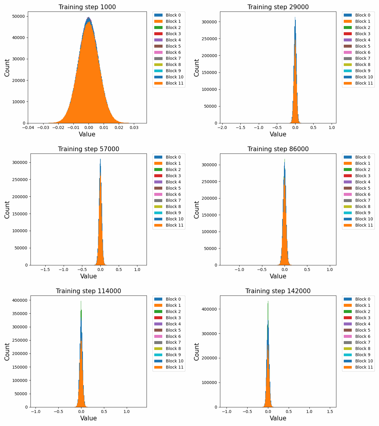
It is possible that this shift is simply the model weights adapting to the data distribution (which is presumably roughly Zipfianly distributed) and may be closely related to the initial very steep decreases in loss that are observed. 

The fact that the shift is so early strongly implies that this logistic distribution is in some sense the ideal distribution for the weights and perhaps that a Gaussian initialization does not provide an optimal inductive bias for learning Zipfian data.

However, as a counterpoint, the weight histogram for the attention output matrix does not change to this logistic shape and remains mostly Gaussian throughout.
 

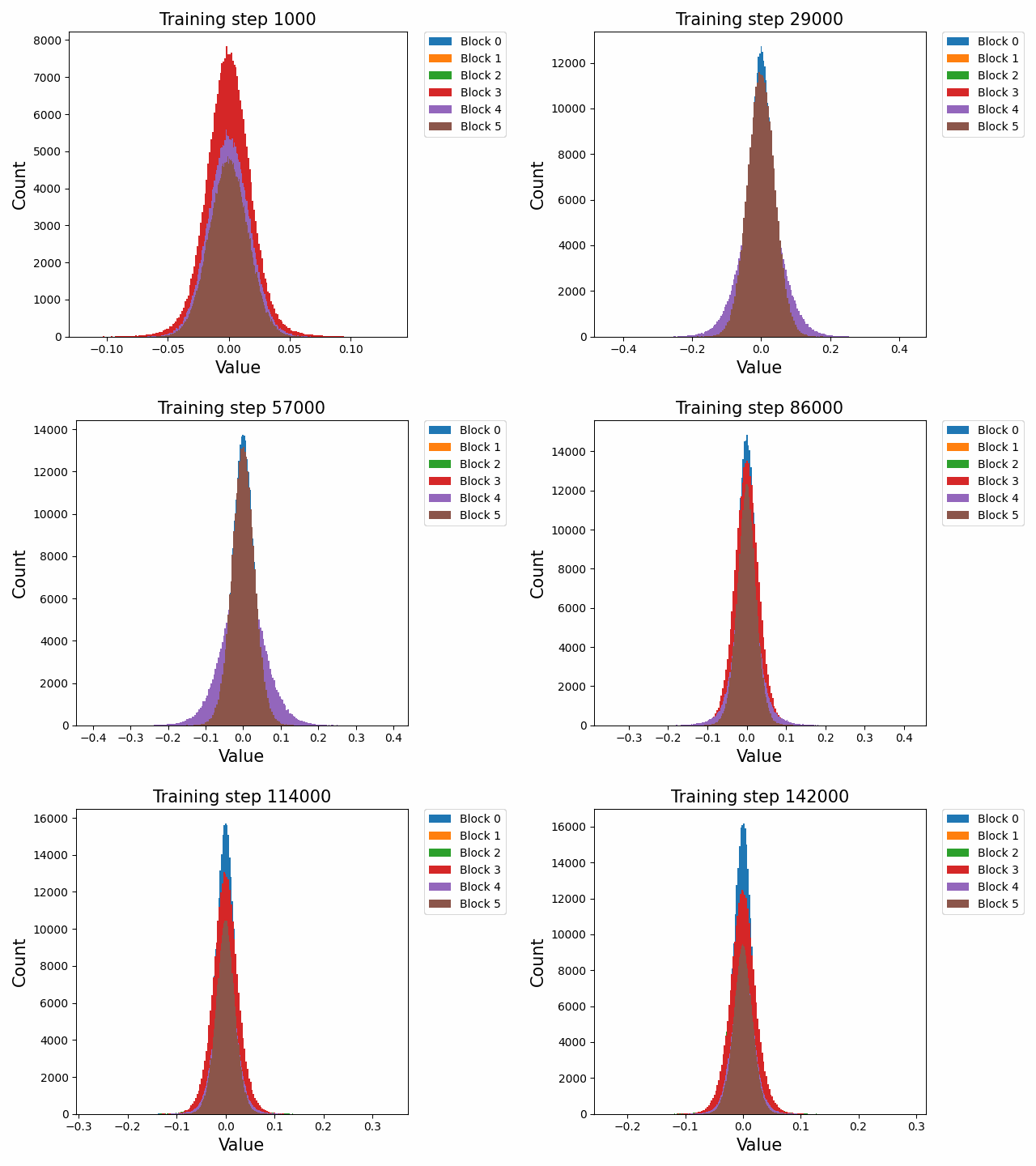
The outliers of this weight matrix also remain fairly small in magnitude compared to the other weight matrices in the network, for reasons that are unclear. The unique status of the attention output matrices can also be seen in their singular value spectrum which is studied later. 

To show the change of distribution in a more quantitative sense, we created animations of the quantile-quantile (QQ) plot of the weight histograms plotted against an ideal Gaussian and an ideal power-law, to show the evolution of the distribution through training. In general, what we observe is that the weight distribution tends to start off Gaussian but develops heavy tails which make the fit eventually very poor. The power-law fit never works particularly well, which is surprising given the power-law nature of the data, and there are significant outliers at the tails which even the power-law does not catch. 

For instance, here is the QQ plot for the attention QKV matrices for the 125M model.

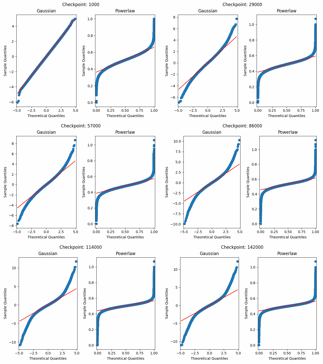
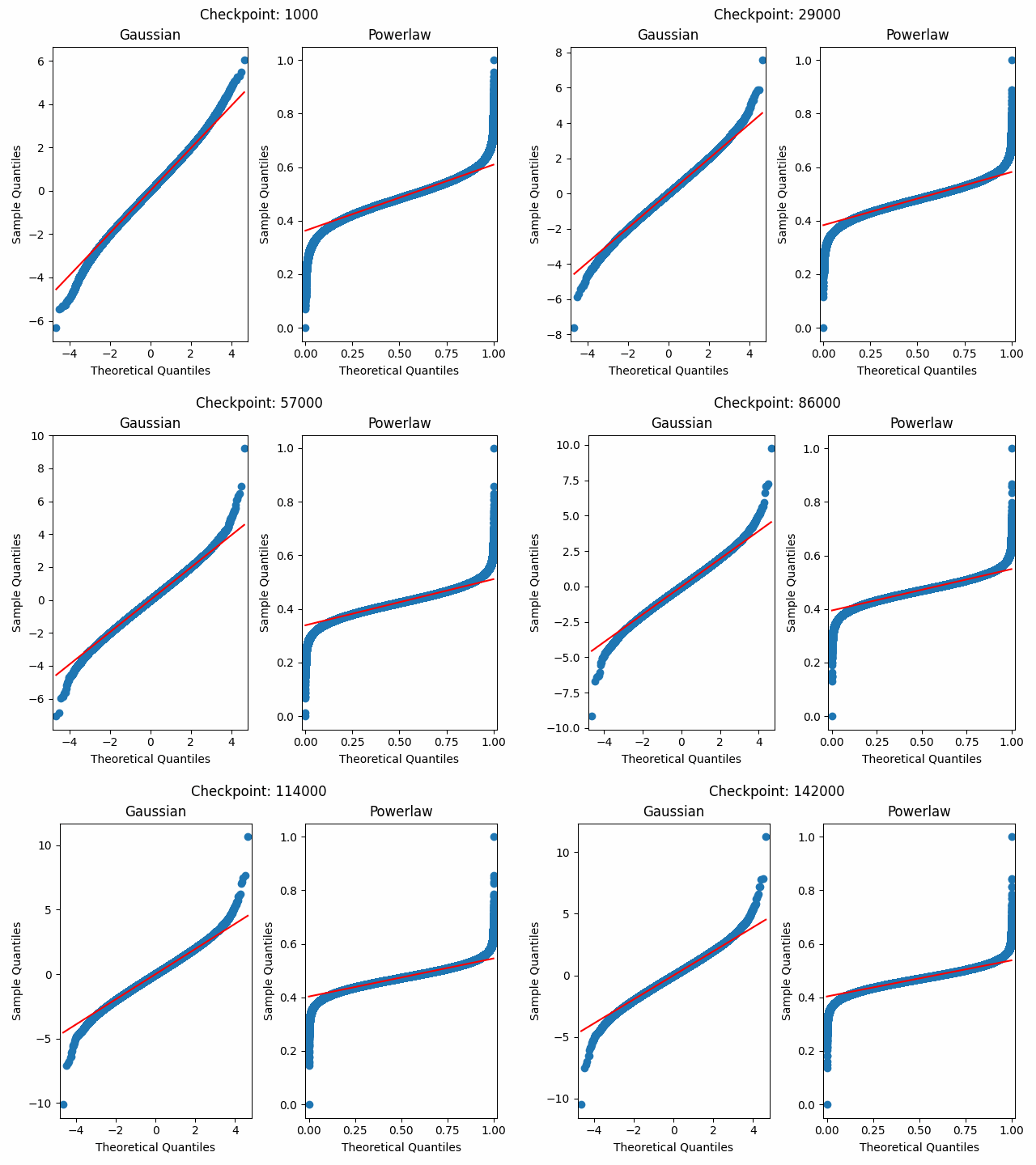
In our preliminary experiments fitting distributions and looking at QQ plots for various distributions, we found that the actual weight histogram is not well characterized by any specific distribution. For instance, it has extremely heavy tails – more so than even a logistic or a power-law distribution, but that the majority of its bulk looked mostly Gaussian. The divergence from Gaussianity also depended strongly upon which weights were being studied. We found that the attention QKV matrices above had the strongest outliers, while the attention dense remained fairly Gaussian throughout training with much lighter tails than the other weights.

Attention Dense for 125m

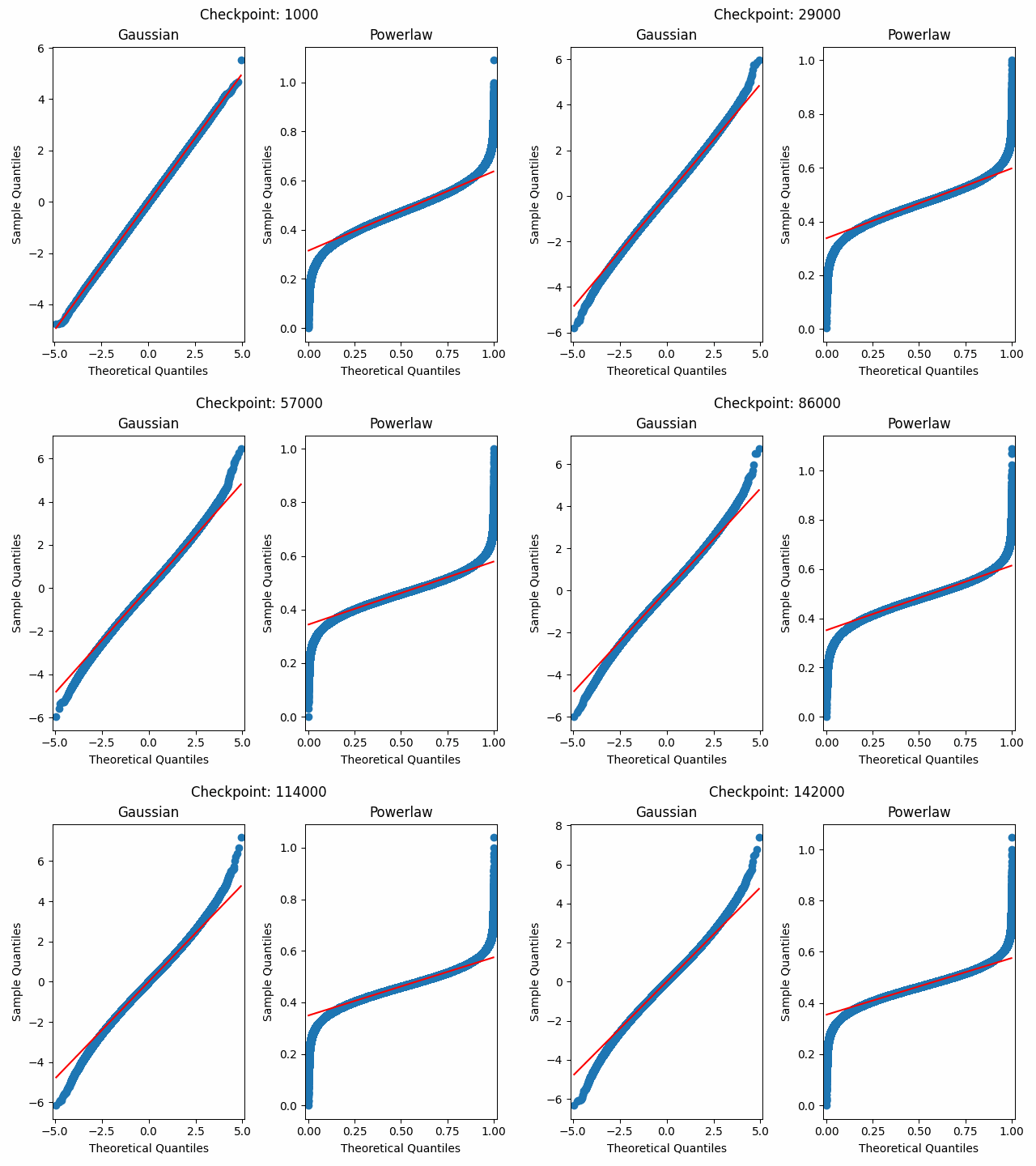
Finally, we studied the MLP weight histograms. Here again we find strong evidence of initial Gaussianity followed by slow developments of outliers at the tails of the distribution

FC in 125m

So do residual stream and weight gradients

We also tested a similar hypothesis for the residual stream and gradient activations during training through the model. These distributions show very similar behaviours to the weight histograms in that they rapidly shift from a Gaussian-ish initial distribution to appearing highly logistic. However, the scale of the outliers is so much greater than in the weights. Moreover, these outliers do not appear to be simply drawn from a heavy tailed distribution but are much more extreme than that, leading us to suspect that either they are the result of numerical instability or issues within the network or else they are deliberately created by gradient descent to serve some specific functional role. More specifically, we hypothesize that an interaction between diagonal preconditioning in the Adam optimizer and the layernorms of the transformer tend to produce outlier activations. 

Here we plot the activations through the residual stream in the 125m network during training.

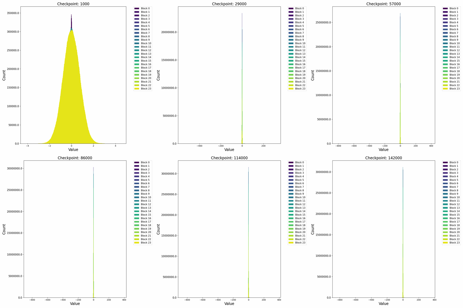
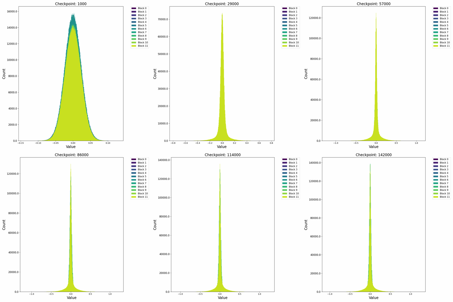
Of note is the relatively sudden shift to the logistic distribution which occurs very early on in training, within the first few thousand steps. This occurred in all of the model sizes that we studied. Very rapidly, the distribution becomes extremely peaked compared to the long tail of outliers that emerge in the residual stream. By about step 40000, we observe that the outlier norms appear to stabilize for the rest of training.

We also investigate how the distribution of the gradients change throughout training. Here we plot the histogram of the gradients of the output MLP weights for the Pythia 125m model.

Interestingly, the gradients show a similar progression to the weights, but much less extreme. They begin as Gaussian, slowly shrink in variance with expanding tails until, at about 20,000 steps, they undergo a sudden shift to a logistic distribution. However, the tail magnitude is much more similar to the weights than the activations, implying that the outlier dimensions are not created by single outlier gradient updates but must instead be the accumulation of a large number of gradient steps.

Residual stream outliers grow rapidly then stabilize and decline

To understand better the dynamics of outliers in the residual stream, we explicitly plotted the maximum absolute values in the residual stream activations on a randomly sampled batch of data from the pile. We found that there was a consistent pattern across model sizes of the outlier norms increasing rapidly during the beginning of training, then cresting and slowly declining. This is the same pattern that we observe later in the MLP weight norms and many other norms throughout the network. Clearly these phenomena should be expected to be related since outliers are presumably propagated into the residual stream through anomalously large weight norms.

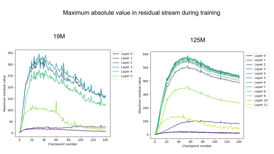
Interestingly, for the larger 125M parameter model, we observe that the peak and crest of the residual stream norms occurs later during training and the fall-off is less steep. Also notice that the y axis is not the same and the scale of the outliers is much larger in the larger model, potentially implying that we should expect maximum outlier norms to scale with model size. An additional interesting point is the consistent ordering of the outlier norms by blocks. The first few blocks always maintain extremely low maximum norm throughout training – implying no outlier features. Moreover, the residual stream in the final layer appears to have few outliers as well, and the norm declines to almost baseline levels by the end of training. This is likely because the model does not ‘want’ to propagate outliers into the de-embed. 

To further, elucidate the block-wise structure of the residual outliers, we also plotted the maximum outlier norm ever observed in each block across training.

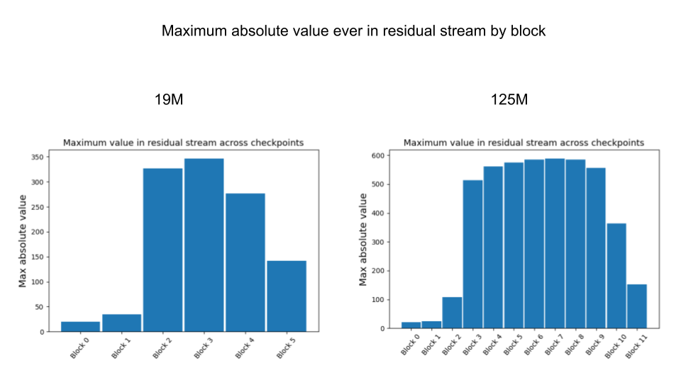
We observe that there is clearly an inverted U shape in the outlier norms as they propagate throughout the network. They begin with relatively low norm – probably roughly equivalent to the rest of the residual stream – in the first two blocks. By blocks 2-3 they have fully formed and then propagate through the rest of the network with approximately the same maximum norm until they reach the final few blocks where their norm rapidly decreases back in line with the rest of the residual stream. This decrease is probably necessary so as to avoid the outliers having massive impacts on the decoding which is a linear readout of the residual stream at the final block (albeit passed through a final layer norm). However, if the outliers can be precisely controlled by the network in this way, it suggests that they are in some sense a ‘deliberate’ creation of the network to perform some specific computational function rather than an accident of the numerics. 

MLP Weight norms rise, peak, and fall

If we plot the evolution of the norms of the weights during training for the MLP blocks (both FC_in and FC_out), we observe a highly consistent pattern of the norms increasing rapidly from initialization, peaking somewhere between checkpoints 20-40 and then declining after that. The degree of decline decreases with increasing model scale, to the point where it looks more like an asymptote for the largest 1.3B model.

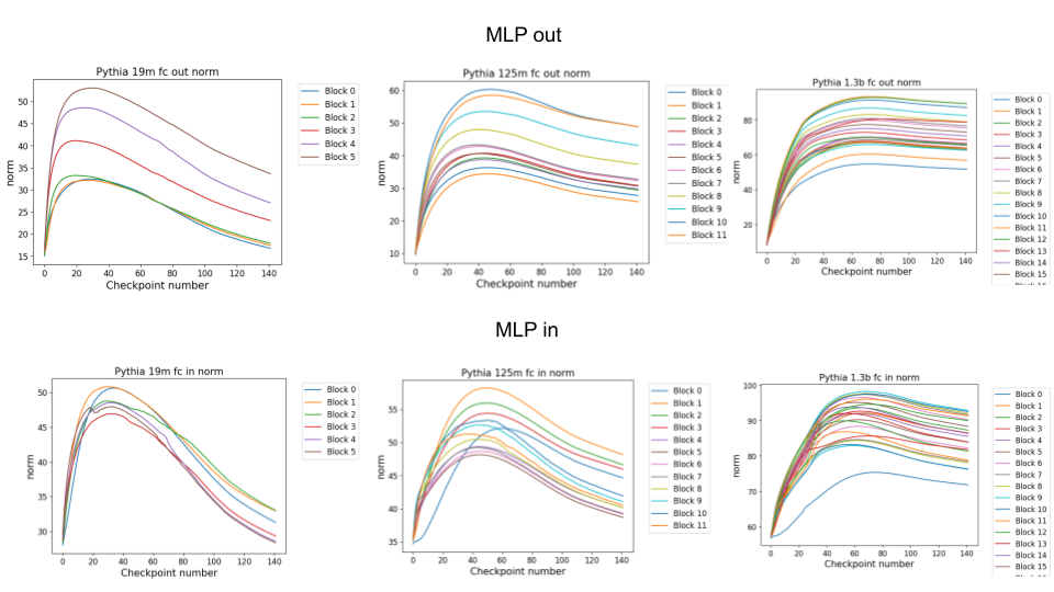
We hypothesize that this effect is due to weight decay in the network. At the start, the network weights are initialized to far below the ‘characteristic’ scale required to process the data correctly, leading to rapid growth. Once the representations have stabilized and the network is at the right scale, then the weight decay forces the network to find ways to decrease the weight norms while maintaining performance. It is unclear how exactly this occurs. One hypothesis we have, which relates to our later findings, is that the model finds a way to ‘cheat’ the weight decay by simply decreasing the weight norm and increasing the layernorm weights or biases because weight decay is not typically applied to the layernorm parameters.

Interestingly, the timing of this decline appears to occur also around the time that the weight distribution is observed to shift from being Gaussian to being more logistic and heavy tailed, indicating that perhaps these two shifts are related or different manifestations of the same underlying change. With this analysis, we cannot definitively show this, however. 

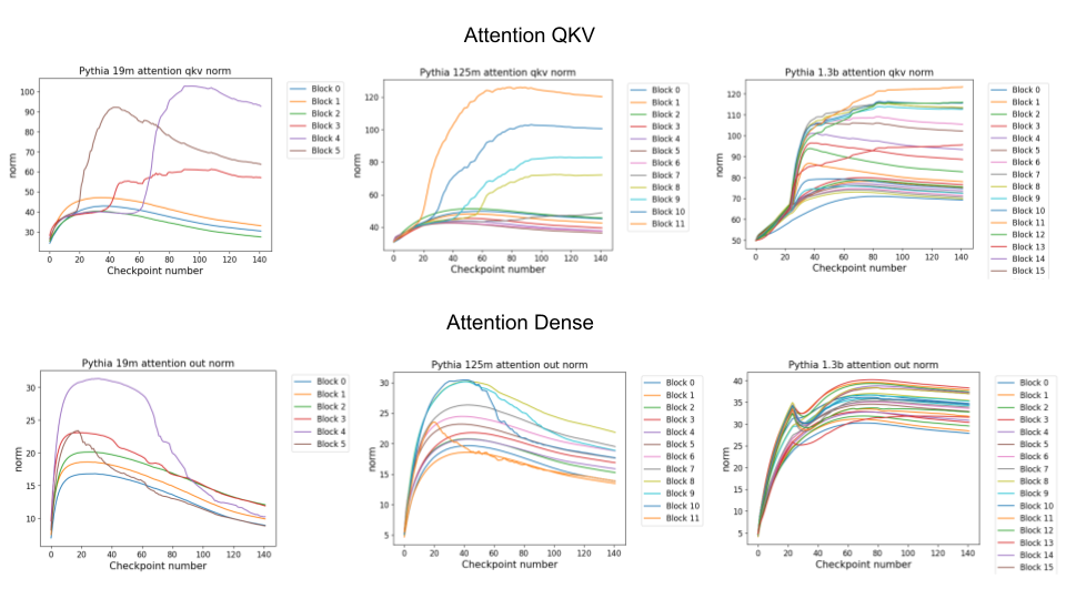
If we perform the same analysis with the attention weights, we observe broadly similar patterns but with much greater variability between blocks. Here, we observe that, especially in the smaller models, there are some blocks with high and rapidly growing norms that asymptote and decline and other blocks appear to have a much more measured growth pattern. This is especially true of the attention QKV norms where it is possible to see that the final blocks appear to grow to much larger norms than the earlier blocks. The reasons for this is unclear but it occurs reliably across model scales. 

MLP biases increase and asymptote

Robustly across model sizes and blocks we observe that the biases in the MLP blocks increase and then asymptote at significantly higher values than the initialization. We believe this indicates either that the ideal scale of the network is much higher than the typical zero initialization, or that the biases are being used in some unusual way to combat weight decay on the weights. The consistency of this effect is impressive. The only exceptions to these are in the FC_out norms for the smaller pythia models which appear to show a small decline like the weight norms. The bias norms are also interesting for appearing to show a greater difference between different blocks.

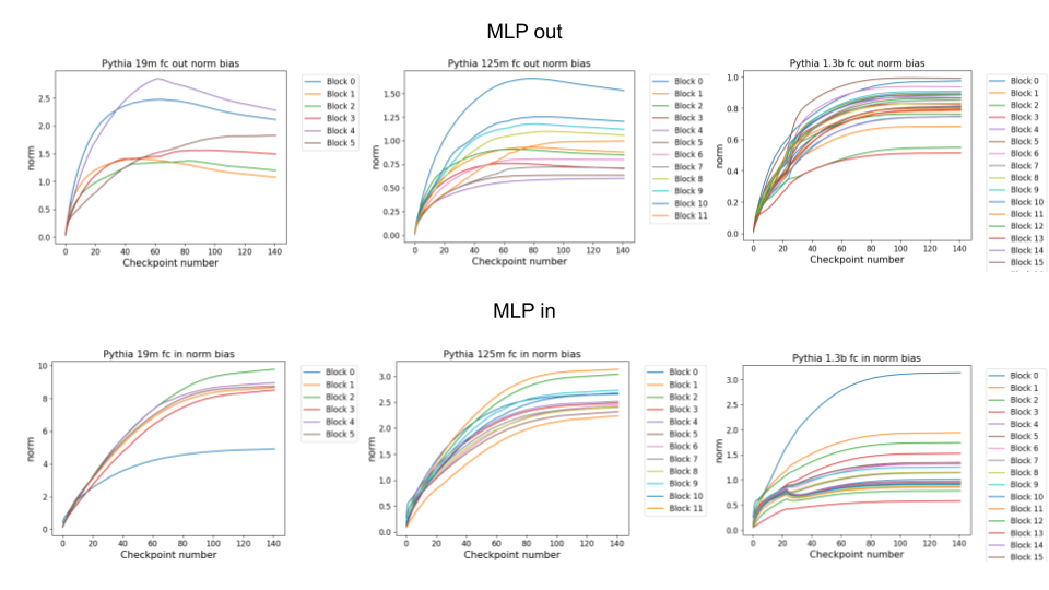
In general, the smoothness of these changes during training is highly surprising. This means that it might be possible to fit these curves to predict general norms of various weight and bias matrices later on in training or after training. It is also possible that the fact that these measures have often clearly not fully asymptoted or come to some equilibrium value indicates that the Pythia models are still undertrained and that further training would be helpful.

Layernorm weights and biases

We perform the same analysis of the layernorm weights and biases throughout training with the results plotted below,
 

What we observe is that the layernorms exhibit qualitatively different behaviour from the MLPs and attention weights. The layernorm weights can both increase and decrease during training where typically the weights will decrease for block 0 (i.e. in the embed) and then increase for later layers in approximate order of depth of the layer. There is also some interesting non-monotonic behaviour especially with the smaller layers although most changes in the 1.3B model appear highly smooth. 

When studying the biases, on the other hand, there is an almost monotonic increase in the bias norms throughout training. There is, however, a wide dispersion of the norm increases with some blocks barely increasing in norm at all while other blocks increase substantially. Again, this increase appears to be in approximate order of depth, with block 0 and early blocks increasing substantially and later blocks increasing less. This may be important for countering the effects of weight decay or else ensuring that the early residual stream and outputs of the embedding matrix are of a sufficient norm to allow easy processing for the rest of the network.

Euclidean Distance from initialization during training

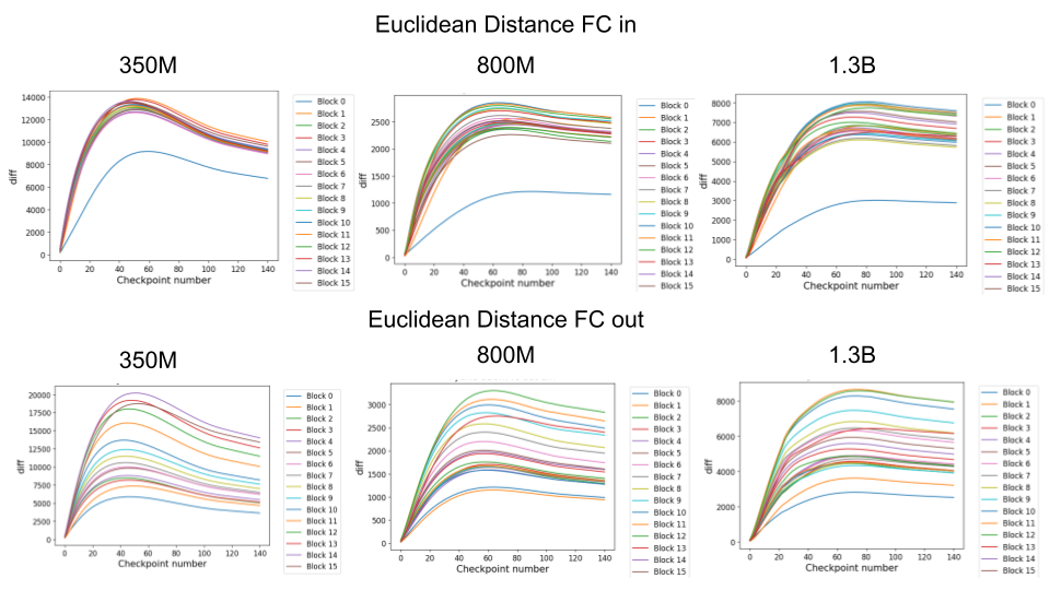
As well as studying the norm, we thought it might be interesting to study the direct euclidean distance between the initial (at checkpoint 0) and final conditions of various weights. This may give us a better indication of how much weights actually ‘move’ during training.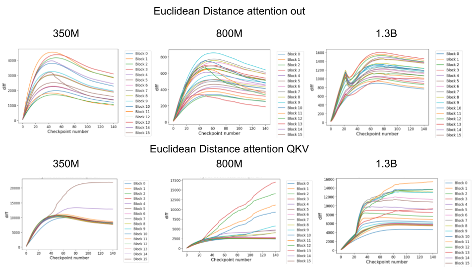

Some of the weight blocks had euclidean distances that very closely tracked the norms. For instance, the attention out weights had the classic rapid increase and then slow decline phase that we see in the weight norms. Interestingly, even here the 1.3B model appeared to show an unusual phase-shift at around 20 checkpoint steps in its euclidean distance. Moreover, for all models the peak of distance from initialization appeared to occur at between 20-40 checkpoint steps, perhaps indicating that this time is significant.

For the attention QKV weights we observed very different apparent behaviour between different models, for reasons that we do not understand. All of the models seemed to exhibit discontinuous behaviour at around checkpoint step 20, but in different ways. 350M and 1.3B appeared to exhibit sudden distance increases for some blocks only at starting at checkpoint 20 which then asymptoted to a final value. By contrast, the 800M appeared to have a constant monotonic increase in distance for a select few blocks which began diverging at checkpoint 20 but does not asymptote. We are unsure of why checkpoint 20 seems to be of such importance here. We conjecture that it may be to do with the learning rate schedule – potentially checkpoint 20 is when the learning rate warmup finishes or when there is some other large change in schedule. Alternatively, this divergence could be related to some intrinsic dynamics throughout training. Noticeably, in many of our plots, we observe that things rapidly change and often tend to asymptote or phase shift to a different behaviour between checkpoints 20 and 40. These include, the weight norms, the embedding norms, and the norms of outliers in the residual stream. These plots may suggest that at least for some observables training can be split into two phases – a ‘rapid learning’ phase where the observables rapidly adjust and then a slow refinement phase where norms asymptote or slightly decline. This is highly speculative however and it is unclear to what extent these changes in norms affect the development of more low-level representations in the network.

If we plot the distance from the initial checkpoint for the MLP blocks, we notice much smoother behaviour that is much more similar to the behaviour of the norms. Specifically, We observe a rapid rise in distance, which peaks between checkpoints 20-40 before declining or asymptoting. All models appear to show qualitatively the same behaviour here, although there perhaps may be an effect where smaller models show greater declines in distance than larger models which instead seem to asymptote directly rather than decline. Also of interest is the outlier behaviour of block 0 in the FC in MLP which changes much less than others. We believe this is because due to the parallel attention and MLP in GPTJ structured networks, Block 0 is best considered an extension of the embedding matrix, since it is applied directly to the embeddings before any attention or nonlinearity has been applied.

Analysis of de-embed and final layernorms 

As well as the standard MLP and attention blocks, of significant importance to the actual output of the model is its de-embedding matrix and final layer norm, and we analyze these separately. Unlike GPT2 models, which use a tied embedding and de-embedding matrix, in GPT-NeoX based models these are learnt separately. The norms of the de-embedding matrix (left) and final layernorm (right) are plotted below,

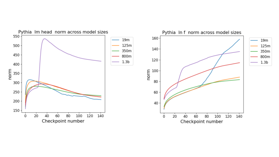In general, we observe that these norms are highly idiosyncratic depending on the model size, and that there often is not consistent behaviour across scales. For instance in the final layernom, there appears to be a pattern of increasing norm with scale except for the highly anomalous behaviour of the 19m model which appears to begin half way through training. Similarly, the highly anomalous behaviour and rapid growth of the de-embedding norm in the 1.3B model appears only after 20000 steps. It is unclear if these behaviours are in some sense ‘natural’ or are the result of idiosyncrasies or instabilities during the training process.

Tokenizer Embeddings are rapidly learnt then stabilize

Transformer language models utilise an embedding matrix which maps the initial one-hot encoded token to the dimension of the residual stream. These embedding matrices are typically learnt during training, so that essentially the model begins with a learnt linear map which can construct the initial vector space in which the tokens are located. Here we are interested in how this embedding space is learnt during training.

We plot the first 256-256 dimensions of the correlation of this embedding matrix $E{E}^T$ where $E$ is the embedding matrix. This correlation matrix describes how correlated specific token embeddings are with each other. Here we plot the first 256 dimensions because these are hardcoded to the ascii characters in the Pythia tokeniser and so a rich structure is present. If we plot the evolution of this matrix over training we obtain the following:

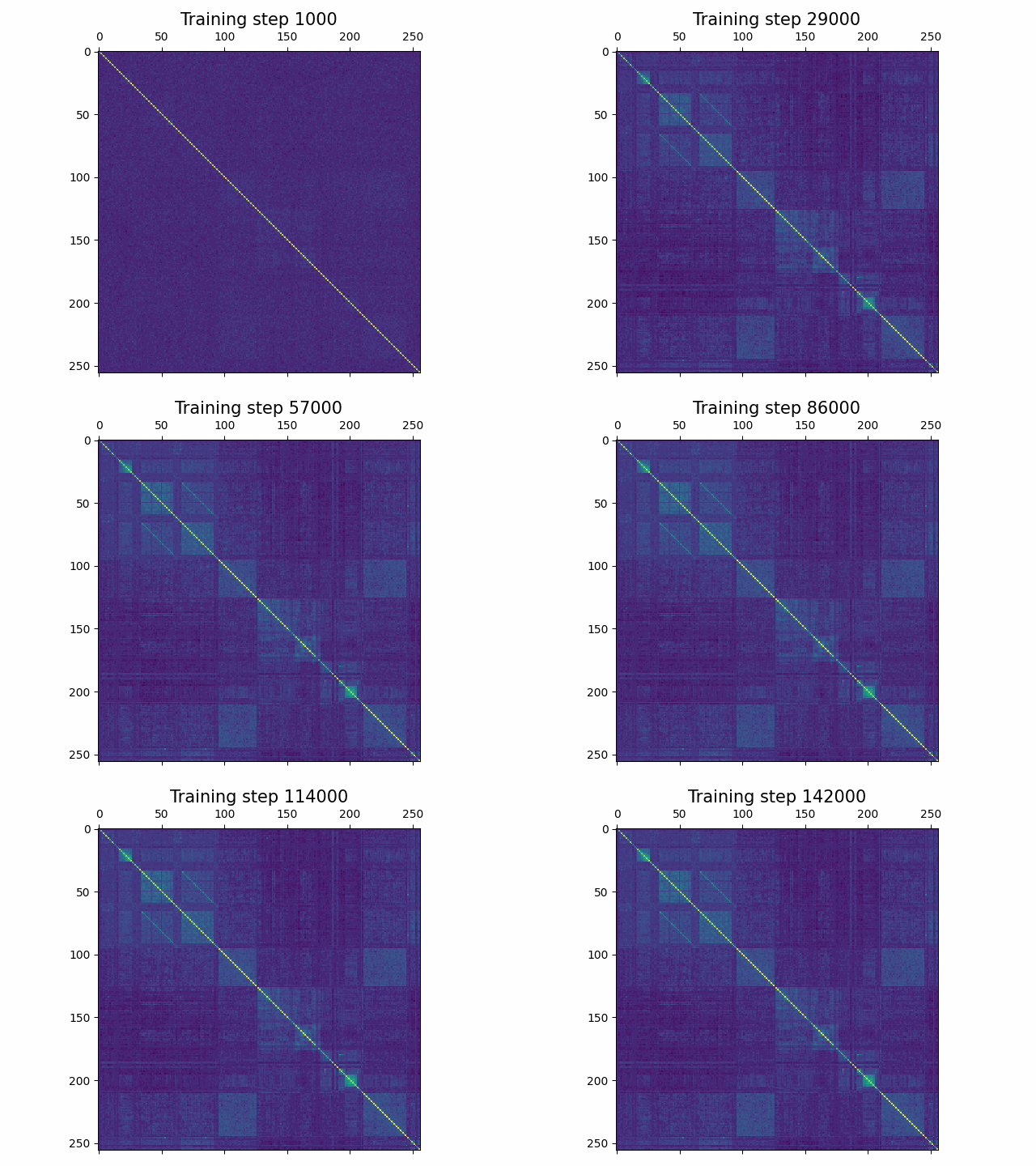
We observe that the embedding matrix successfully learns a rich correlational structure between the first 256 tokens. Several clearly structured regions are visible. For instance the most leftward block represents the numbers 1 to 9. Then the next four blocks represent all of the ascii letter token a…z and A…Z both with and without leading spaces. The fact that the model learns such systematic embeddings shows that it can pick up on relatively coarse correlations within the embedding matrix and use these to learn a coherent and consistent embedding space. If we zoom out beyond the 256 dimensions, the tokens are instead set by the BPE algorithm and all apparent structure disappears. This is likely because the BPE algorithm is not guaranteed to tokenise into some interpretable order and hence the correlation matrix looks randomised. We think it is likely that there exists some permutation of the embedding matrix that would reveal this structure again but have not experimented deeply with finding it.

Also of note is that the model very quickly learns this structure and it stays very stable throughout training. It is possible that a significant amount of the initial loss decrease comes from simply learning this good structure of the embeddings and where the model essentially starts out as a linear auto encoder (with the embedding and de-embedding matrix) of the data.  After that the structure changes slowly but is broadly consistent.

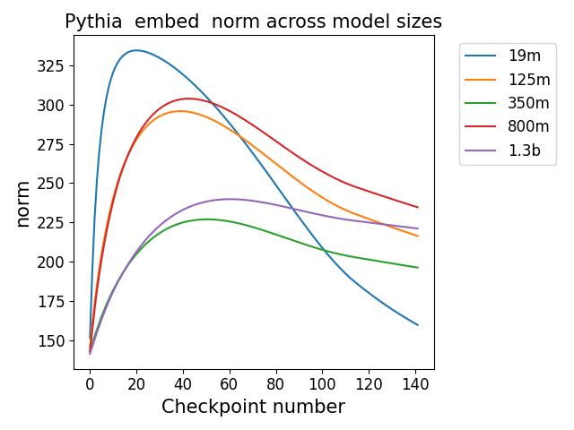
If we plot the norm of the embedding matrix across different model sizes during training, we observe a very similar pattern to the MLP blocks of a rapid rise followed by a slow decay of the norm, presumably driven by weight decay. Interestingly, the norm patterns do not appear to be homogeneous with scale but vary significantly between the different models. 

Power law weight spectra but differing behaviour across components

In the previous post, we showed that the singular values of the weights of GPT2 models had a highly consistent power law spectrum when plotted on a log-log scale. This differs substantially from the Gaussian initialization of the weights, implying a consistent distributional shift towards heavier tails between the start of training and the end, which was also supported by the heavy tailed histogram distributions of the weights.

Using the Pythia checkpoints, we can observe this shift to power law behaviour occurring during training. Interestingly, we see more evidence for Gaussianity in the final weights in the Pythia models than in the GPT2 models. We are unsure exactly what this indicates. Gaussianity is indicated by a highly ‘flat’ singular value structure with a relatively slow and steady fall of. 

We observe different behaviours between the weight matrices of different components of the model. For instance, the MLP weight spectrum undergoes a substantial reorganization into a power law structure during the first checkpoint which it then maintains throughout training with relatively little change. There are also significant differences between block 0 and the later blocks. This was not observed in the GPT2 models.  We hypothesize that this occurs because the Pythia models follow a GPT-Neox structure of the attention and the MLP block being in parallel in the residual rather than sequential. That is, the standard GPT update is $x^{l+1}=x^l+ffn\left(attn\right(x^l\left)\right)$ where the MLP is in series to the attention. The GPT-Neox structure, on the other hand places them in parallel: $x^{l+1}=x^l+attn\left(x^l\right)+ffn\left(x^l\right)$ which means that the first MLP block is not affected by the attention and is essentially an extension of the embedding matrix, leading to its divergent behaviour.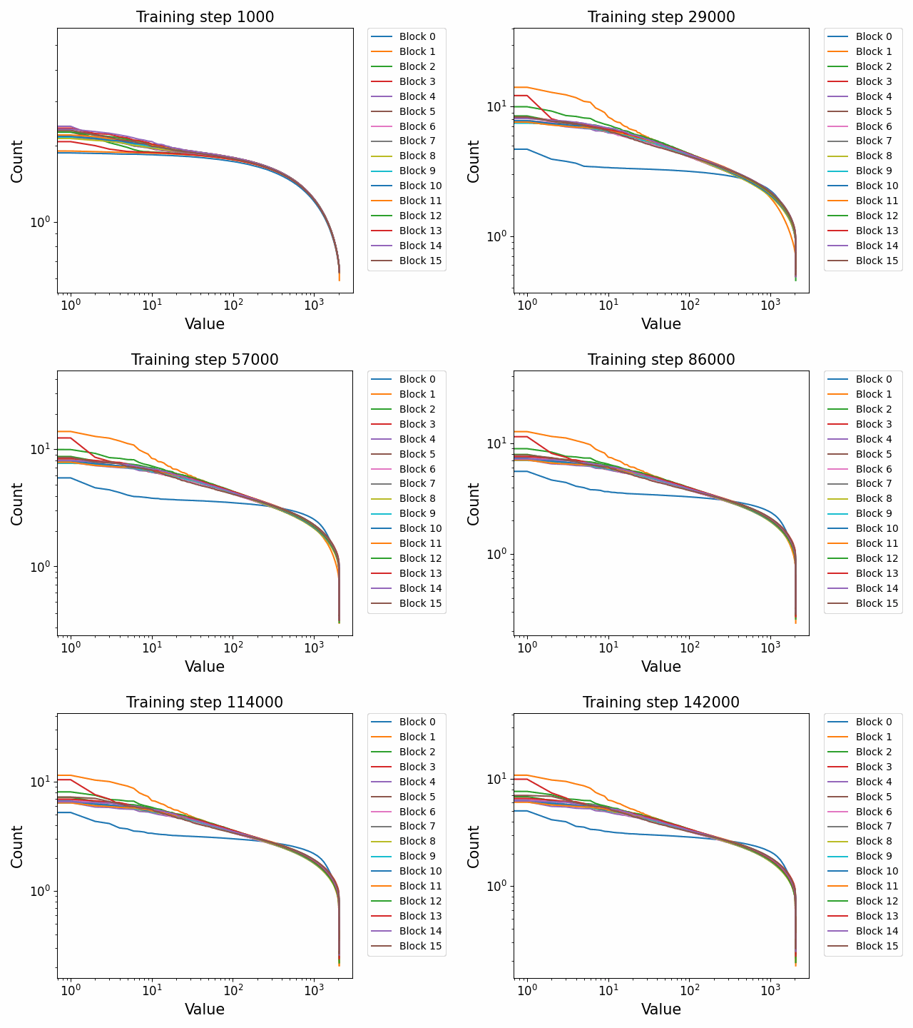

Unlike the MLP blocks which appear to develop power-law like behaviours early on, we notice that the attention_dense weight spectrum appears to remain very close to Gaussian (albeit with fluctuations) throughout training. 

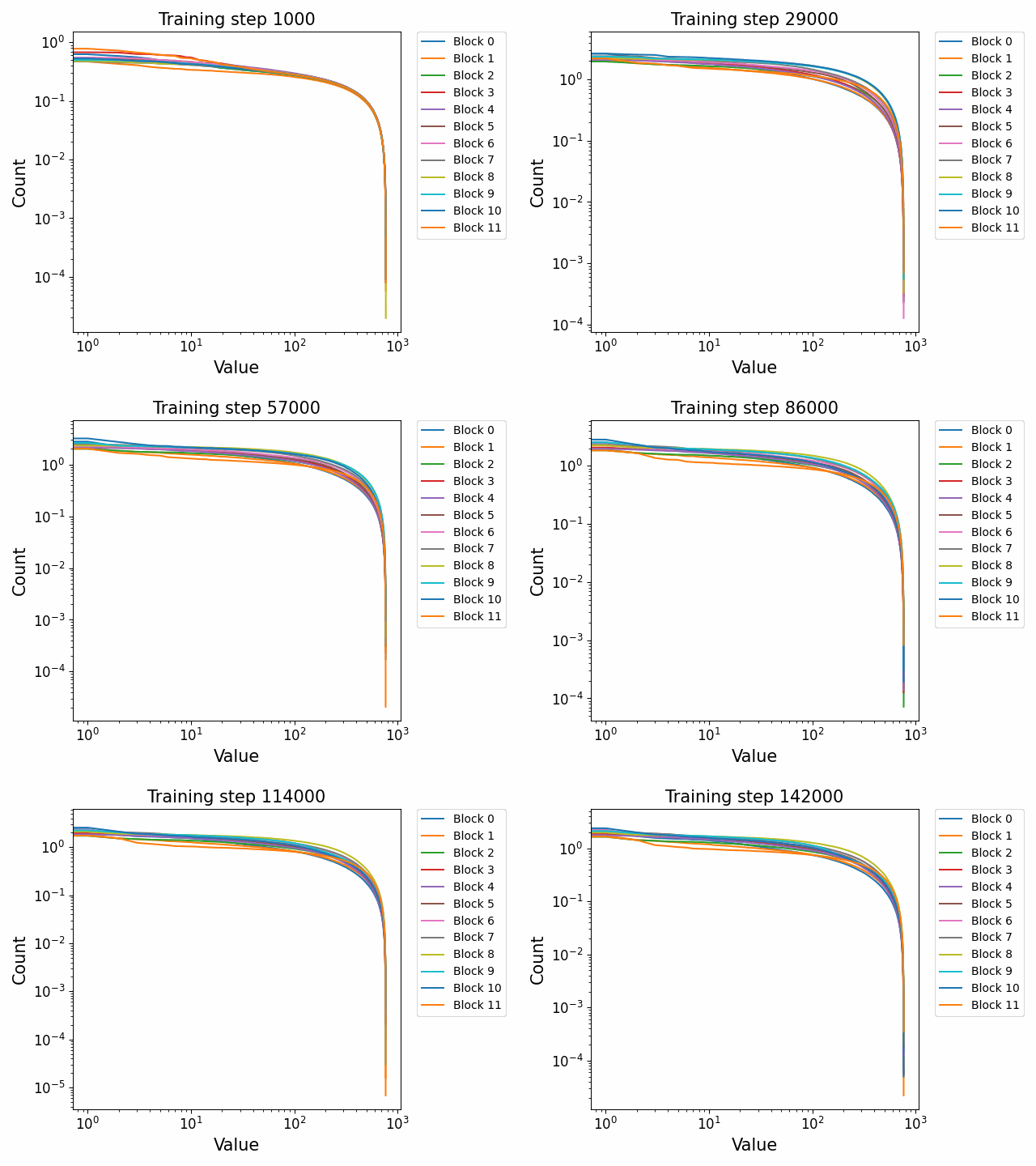
This may imply that these weights are not sufficiently trained due to poor conditioning or else that this is in some way the optimal behaviour for them.
 

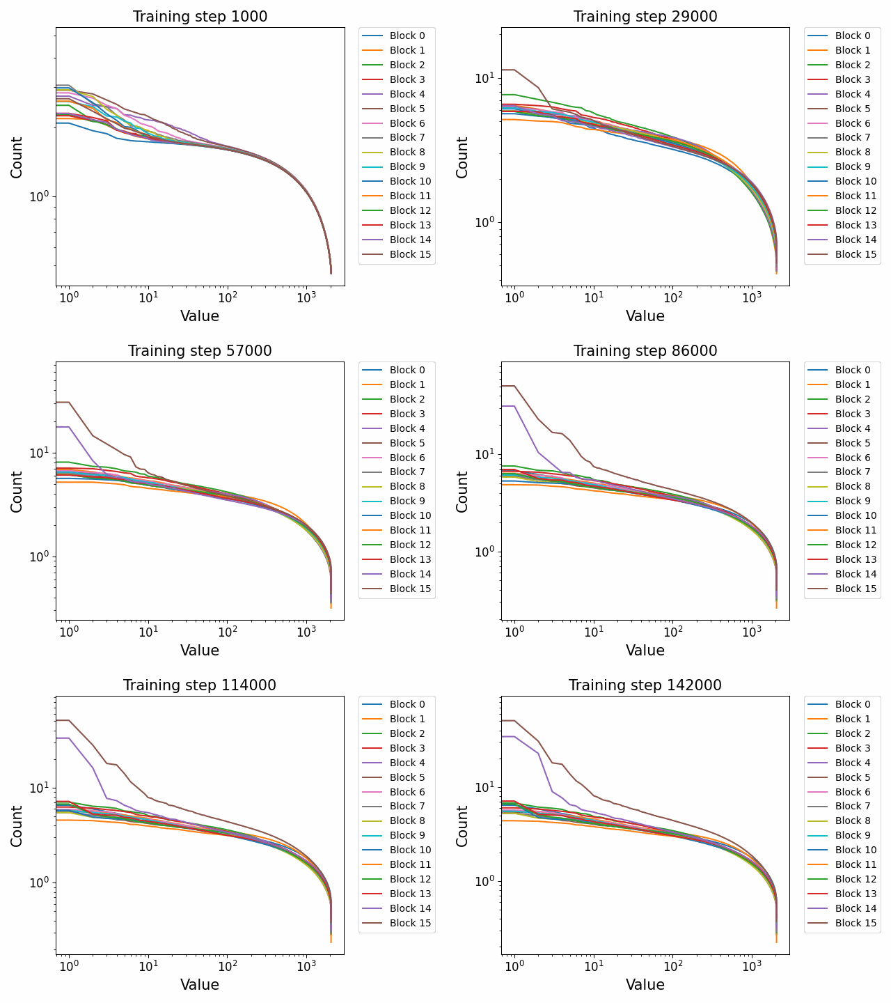
In the attention QKV weights, we observe a highly interesting effect where some blocks develop consistently high ‘outlier’ singular vectors and overall a much heavier tailed power-law curve than others. The outliers develop only in the attention QKV weights and not the other weights. Exactly which blocks show this behaviour appears to differ between different model sizes and does not show consistent behaviour. These outlier blocks appear to develop consistently throughout training including in the later stages of training. This is distinct from the simple formation of the distributional structure which occurs early and then does not shift much throughout the bulk of training. 

Plotted are examples of the QKV weights for the 125m and 350m models: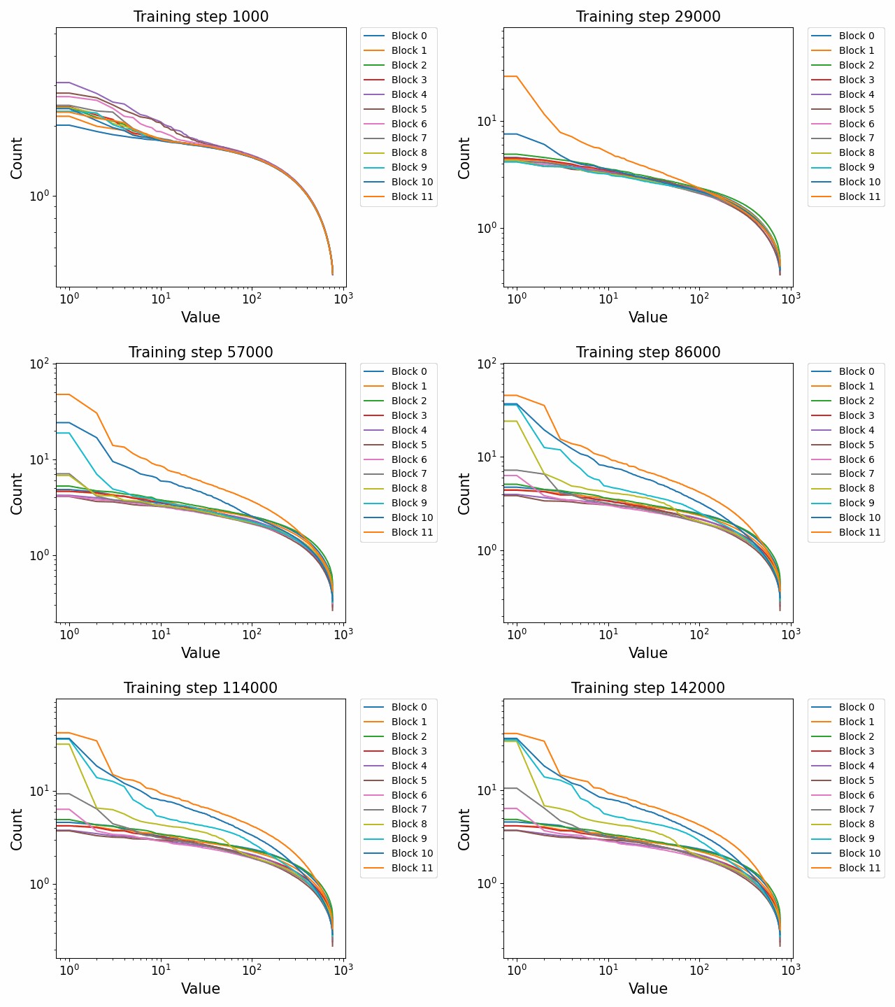
 

Closeness to final SVD direction vectors grows exponentially and develops late

Given the seeming success of using the SVD directions [LW · GW] to try to understand the processing that occurs in the MLP layers and OV circuits of transformer networks, it is also interesting to try to understand when and how these SVD directions develop during training. To do so, we first confirm that many SVD directions remain interpretable in the Pythia models (an interesting fact that shows that the results generalize beyond the GPT2 family of models although the SVD directions are generally cleaner in the GPT2 model family).

Secondly, we compare the SVD direction strings (the top-20 tokens for the top-30 singular vectors) for each of the Pythia model sizes across each of the checkpoint steps for each of the MLP and OV circuits to the final svd directions. If we plot both the number of exact matches, we observe that the similarity of the SVD directions to the final direction emerges very late in training and appears to increase exponentially towards the end. This means that either the SVD directions themselves are relatively unstable during training or that the final representations are only formed close to the end of training in a way that is interpretable as SVD directions. Example plots across blocks of the SVD direction closeness are shown for different model sizes

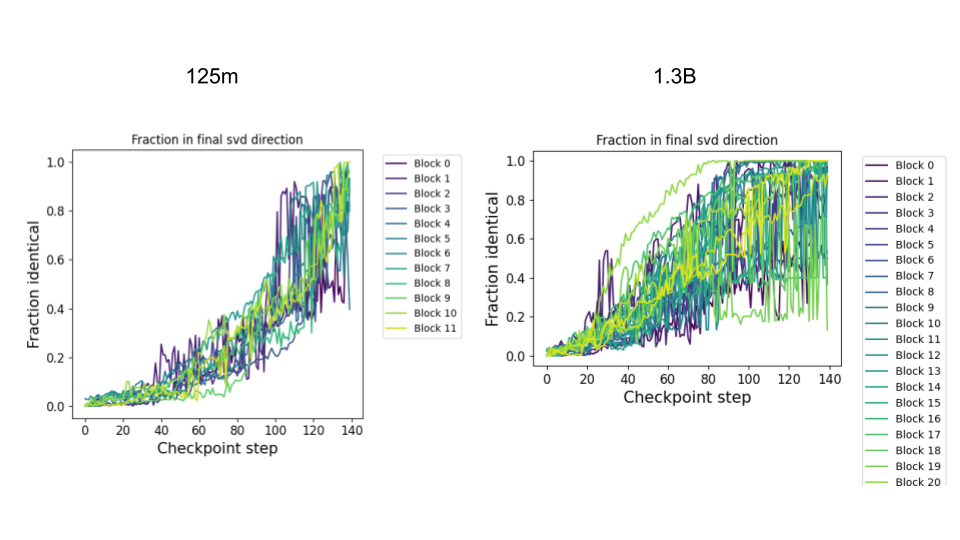Generally, we observe that larger models have more stable SVD directions across checkpoints. Either indicating that they are better trained and so form good representations, or else that the weight matrices diverge less from their initialization than for smaller models, or perhaps both. This can be seen in the following plot that averages the similarity across all blocks for each model size:

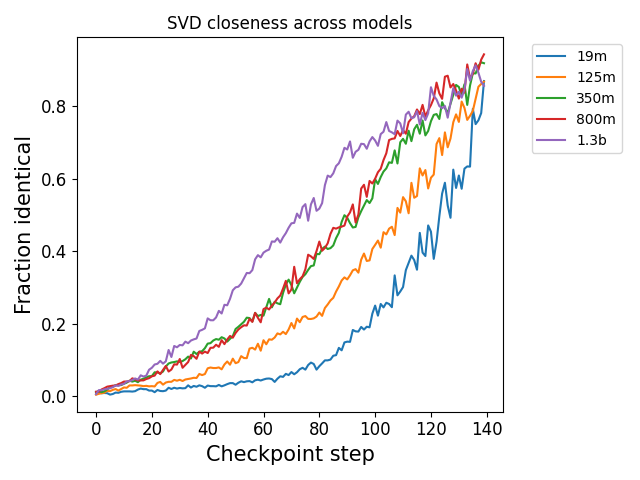
Where we can clearly see a strong effect of scale on the coherence of the SVD directions across training. This may imply that larger models form more coherent and consistent representations earlier than smaller models. Or, alternatively, may reflect that larger models may simply stay closer to their initialization distribution than smaller models.

By manually inspecting some of the SVD directions across checkpoints, we generally observed that the early SVD directions were consistently uninterpretable, and that this persisted for a long time throughout training (much longer than, for instance, the shift into the logistic distribution for the weights). However, eventually interpretable SVD directions did form but would slowly drift in semantic meaning during training meaning that they were not monotonically converging to their ‘final form’. This might indicate that during training there is some amount of representational drift in what specific heads or layers represent. Alternatively it could just mean that the SVD directions is not a great benchmark for this.

Almost all of these effects are consistent across model scales

As a final meta point, we were quite surprised by how consistent almost all of these effects are across model scales. Certainly the broad distributional facts were identical across scales. We hypothesize that this points to fundamental facts about either the model architecture or data distribution which makes certain distributions optimal to form representations out of, or else common patterns

It would be very interesting to do a comparative study across a wider range of model architectures and potentially modalities to see if the same distributional facts occur here. If this is the case then this would imply something very general about either the representations deep networks form or else the domains upon which they see the greatest success.

Interestingly, in a few cases we observed different behaviours in the Pythia models than in the GPT2 models we previously studied. Most of these relate to the anomalous behaviour of Block 0 in the Pythia models which we hypothesize is related to architectural differences between GPT and NeoX models. Understanding how architectural differences between models relate to the properties of individual weights or biases, as well as the detailed representations and circuits that are formed during training remains extremely understudied, where people typically only compare architectures in terms of the final loss achieved. This is despite the fact that the network architectures likely encode very important inductive biases and can make it very easy or very hard to represent specific kinds of circuits. 

Conclusion

In this post, we have studied the basic distributional facts and statistics about the internal weight, activation, and bias statistics across checkpoints using the Pythia model suite. In general, we have found striking commonalities across different model scales in terms of both training dynamics as well as eventual distributional facts, including between Pythia NeoX models and the GPT2 models we previously studied. In general, our animations and plots indicate that training tends to be a smooth process where many trends, such as increases in norm development of outliers, unfold regularly during training. On the other hand, many important distributional facts, such as the development of logistic distributions of activations and power-law spectrum of weights appear to occur extremely early in training, likely during the initial very rapid decrease in loss that occurs as the model matches the basic properties of the data distribution. These properties then remain broadly stable after the first few steps. We hypothesize that these properties represent fundamental statistical or numerical facts about the data distribution which must be matched by the model. 

Alternatively, other aspects seem to develop throughout training and these may speculatively be thought of as either the model adapting to regularization or else it adapting to finer features of the data distribution. These include the increase and then decrease in weight norms as well as the development of outlier blocks in the spectra of attention blocks. The mechanism behind these effects and their importance to the more micro-level representations of the network remains to be understood.

15 comments

Comments sorted by top scores.