Basic Facts about Language Model Internals
post by beren, Eric Winsor (EricWinsor) · 2023-01-04T13:01:35.223Z · LW · GW · 19 commentsContents
  Activations Are Nearly Gaussian With Outliers
  Outliers Are Consistent Through The Residual Stream
  Weights Are Nearly Gaussian
  Except For LayerNorm Parameters
   Writing Weights Grow Throughout The Network And Reading Weights Are Constant
  Gradients Are Highly Gaussian
  All Weight Parameters Show The Same Singular Value Pattern (Power Law)
  Activation Covariances Show The Same Power Law Pattern Of Singular Values
  Dataset Covariance Matrix
None
19 comments
This post was written as part of the work done at Conjecture.
As mentioned in our retrospective [LW · GW], while also producing long and deep pieces of research, we are also experimenting with a high iteration frequency. This is an example of this strand of our work. The goal here is to highlight interesting and unexplained language model facts. This is the first in a series of posts which will be exploring the basic ‘facts on the ground’ of large language models at increasing levels of complexity.
Understanding the internals of large-scale deep learning models, and especially large language models (LLMs) is a daunting task which has been relatively understudied. Gaining such an understanding of how large models work internally could also be very important for alignment. If we can understand how the representations of these networks form and what they look like, we could potentially track goal misgeneralization [AF · GW], as well as detect mesaoptimizers [? · GW] or deceptive behaviour [? · GW] during training and, if our tools are good enough, edit or remove such malicious behaviour during training or at runtime.
When faced with a large problem of unknown difficulty, it is often good to first look at lots of relevant data, to survey the landscape, and build up a general map of the terrain before diving into some specific niche. The goal of this series of works is to do precisely this – to gather and catalogue the large number of easily accessible bits of information we can get about the behaviour and internals of large models, without commiting to a deep dive into any specific phenomenon.
While lots of work in interpretability has focused on interpreting specific circuits, or understanding relatively small pieces of neural networks, there has been relatively little work in extensively cataloging the basic phenomenological states and distributions comprising language models at an intermediate level of analysis. This is despite the fact that, as experimenters with the models literally sitting in our hard-drives, we have easy and often trivial access to these facts. Examples include distributional properties of activations, gradients, and weights.
While such basic statistics cannot be meaningful ‘explanations’ for network behaviour in and of themselves, they are often highly useful for constraining one’s world model of what can be going on in the network. They provide potentially interesting jumping off points for deeper exploratory work, especially if the facts are highly surprising, or else are useful datapoints for theoretical studies to explain why the network must have some such distributional property.
In this post, we present a systematic view of basic distributional facts about large language models of the GPT2 family, as well as a number of surprising and unexplained findings. At Conjecture, we are undertaking follow-up studies on some of the effects discussed here.
Activations Are Nearly Gaussian With Outliers
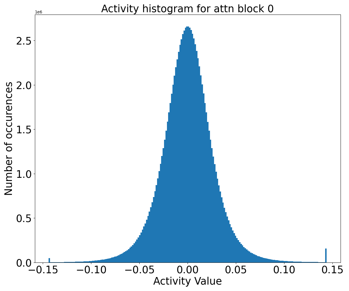
If you just take the histogram of activity values in the residual stream across a sequence at a specific block (here after the first attention block), they appear nearly Gaussianly distributed. The first plot shows the histogram of the activities of the residual stream after the attention block in block 0 of GPT2-medium.
This second plot shows the histogram of activities in the residual stream after the attention block of layer 10 of GPT2-medium, showing that the general Gaussian structure of the activations is preserved even deep inside the network.
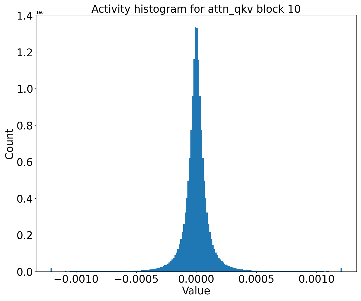
This is expected to some extent due to the central limit theorem (CLT), which enforces a high degree of Gaussianity on the distribution of neuron firing rates. This CLT mixing effect might be expected to destroy information in the representations, as occurs in the NTK limit of infinite width where the CLT becomes infinitely strong and no information can be propagated between layers. It is not clear how the network preserves specific and detailed information in its activations despite near-Gaussian mixing. Particularly, one might naively expect strong mixing to make it hard to identify monosemantic (or even low-degree polysemantic) neurons and circuits.
One very consistent and surprising fact is that while the vast majority of the distribution is nearly Gaussian, there are some extreme, heavy outliers on the tails. It is unclear what is causing these outliers nor what their purpose, if any, is. It is known that the network is sensitive to the outliers in that zero-ablating them makes a large differential impact on the loss, although we do not know through what mechanism this occurs.
Outliers Are Consistent Through The Residual Stream
An additional puzzle with the outlier dimensions is that they are consistent through blocks of the residual stream and across sequences in the tokens. Here we demonstrate this by showing an animated slice of a residual stream (the first 64 dimensions of the first 64 tokens) as we pass a single sequence of tokens through the GPT2-small (red is negative and blue is positive). Here the frames of the animation correspond to the blocks in the residual stream.
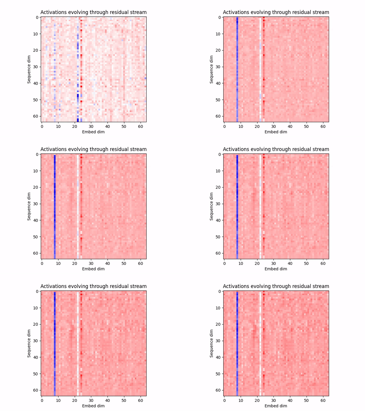
We see that the outlier dimensions (one positive one negative) are extremely easy to see, are highly consistent across the different tokens in the sequence and also across blocks of the network.
It is possible that the outlier dimensions are related to the LayerNorms since the layernorm gain and bias parameters often also have outlier dimensions and depart quite strongly from Gaussian statistics.
We commonly find outlier dimensions across various models and datasets. We are unclear as to why they are so common and whether they are some kind of numerical artifact of the network structure or whether they serve a specific function for the network. Some hypotheses about such functions could be that the outliers perform some kind of large-scale bias or normalization role, that they are ‘empty’ dimensions where attention or MLPs can write various scratch or garbage values, or that they somehow play important roles in the computation of the network.
Weights Are Nearly Gaussian
Similarly to the activation distribution, if you plot a histogram of the weights of GPT2 models (and indeed other transformer architectures), you will see that they are also seemingly Gaussian and, unlike activations, do not tend to have outliers.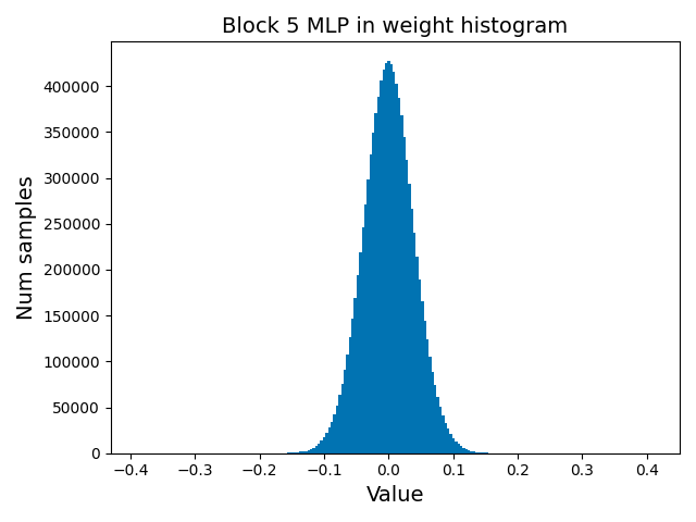
While this is just the plot for the input fully connected layer (FC_IN) in block 5 of GPT2-medium, in practice this pattern is highly consistent across all the weight matrices in GPT2 models.
This is surprising a-priori, since there is no CLT-like explanation for the weights to be Gaussian. One hypothesis is that the weights were initialized as Gaussian and did not move very far from their initialization position during training. If this is the case, it would imply that the loss landscape for these transformer models is relatively benign such that there exists good minima close to random Gaussian initializations. It would also be interesting to explicitly measure the degree to which weights move during training for models where we know the initial state.
A second hypothesis is that, with randomly shuffled data, we should expect the gradient updates to be uncorrelated beyond the length of a sequence. If we are training stably with a low learning rate, then we might expect this uncorrelatedness to dominate the coupling between updates due to moving only a small distance in the loss landscape, which suggests that the sum over all updates should be Gaussian. A way to check this would be to determine if non-Gaussian initializations also converge to a Gaussian weight structure after training.
An alternative hypothesis is that parameter updates during training are subject to a similar (near Gaussian) mixing process as the network pre-activations at initialization. That is, if updates to a particular set of parameters are weakly correlated (within a layer and across training batches), then the parameters may converge to Gaussian statistics. This would mean that many different initializations could lead to Gaussian parameter statistics.
Except For LayerNorm Parameters
An exception to the prevailing Gaussianity of the weights is the LayerNorm Parameters (bias and gain). While they are primarily Gaussian, they share the pattern of the activations where there are also clear outliers. This may be related to or the cause of the outliers in the activation values that we observe. Here we plot the LayerNorm weight and bias parameters of block 5 of GPT2-medium and observe that they look nearly Gaussian with a spread of outliers. This picture is qualitatively different from the activation outliers earlier, which had a couple concentrated outlier values. Instead, the LayerNorm weights look like a sampling of a nearly Gaussian distribution with high kurtosis (4th cumulant or connected correlator). Interestingly, the weight distribution is not centered at 0 but at approximately 0.45 which implies that the layernorm parameters tend to approximately halve the value of the residual stream activations before passing them to the attention or MLP blocks. This may be to counteract the effect of the spherical normalization and mean-centering applied by the layer-norm nonlinearity itself. Also of interest is that most of the outliers, especially for the weights, appear to be left-tailed towards 0. This implies that some dimensions are effectively being zeroed out by the layernorm gain parameters, which could potentially be scratch or unused dimensions?
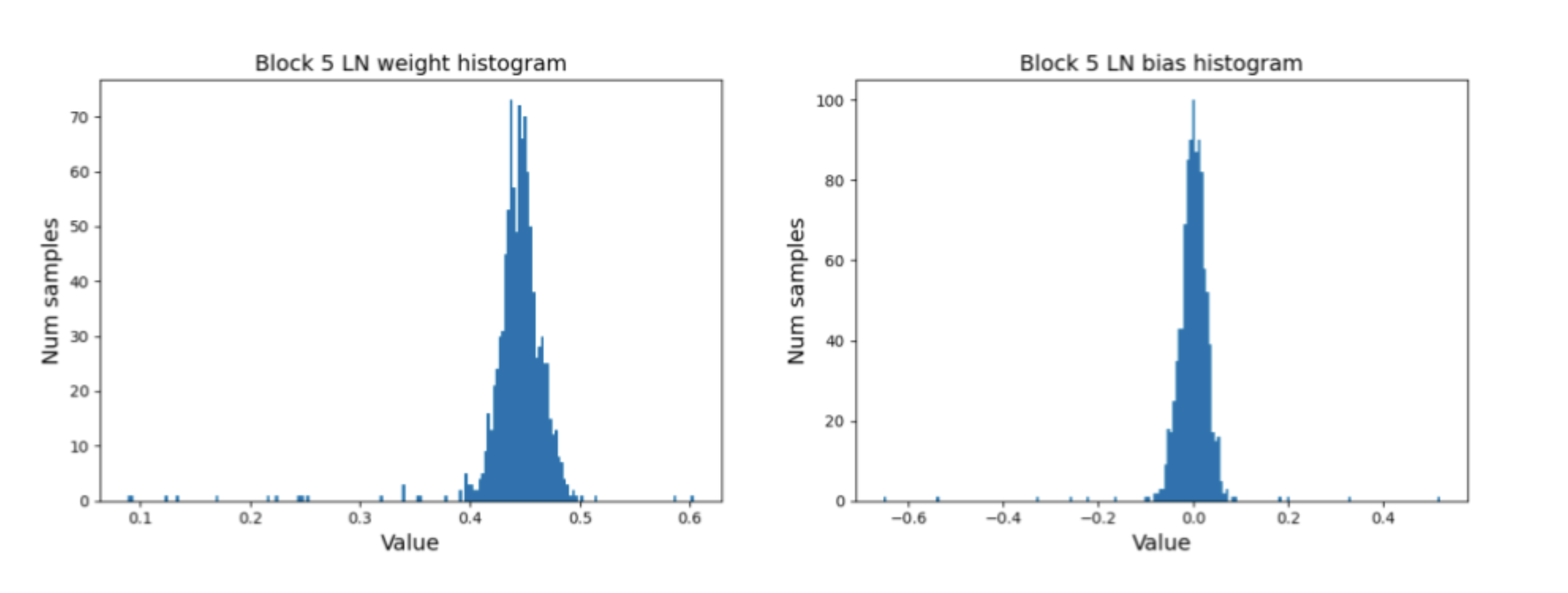
Given that Layer-Norm is a geometrically complex nonlinearity, [LW · GW] it is probably meaningful that the LayerNorm parameters and residual stream activations deviate from Gaussianity in similar ways.
Writing Weights Grow Throughout The Network And Reading Weights Are Constant
An interesting and unexpected effect is visible when we plot how weight norms evolve throughout the network.
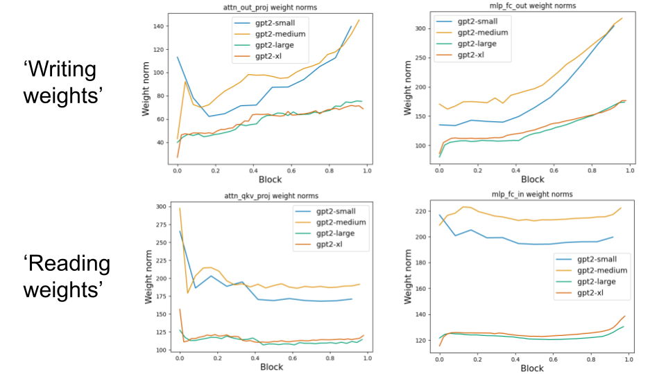
Specifically, we find that the weights that ‘write’ to the residual stream – the O matrix of the attention block and the output MLP matrix appear to grow as we move through the blocks of the network. On the other hand, the ‘reading weights’ – the Q and K matrices as well as the input MLP matrices appear either constant, or start out very large and then quickly drop and remain relatively constant.
Another interesting fact that becomes highly apparent here is that there appears to be a clear divergence within the GPT2 family where small and medium appear to have substantially larger weights than large and XL. Moreover, there also appear to be some differences in behaviour between the two clusters where the writing weights in large and XL do not increase through the network layers to anywhere near the same extent as the small and medium.
Gradients Are Highly Gaussian
Following on from the prevailing theme of Gaussianity, if we look at the histogram of the gradient values for various weights throughout the trained network on dataset examples from common crawl, we see a similar pattern of ubiquitous Gaussianity.
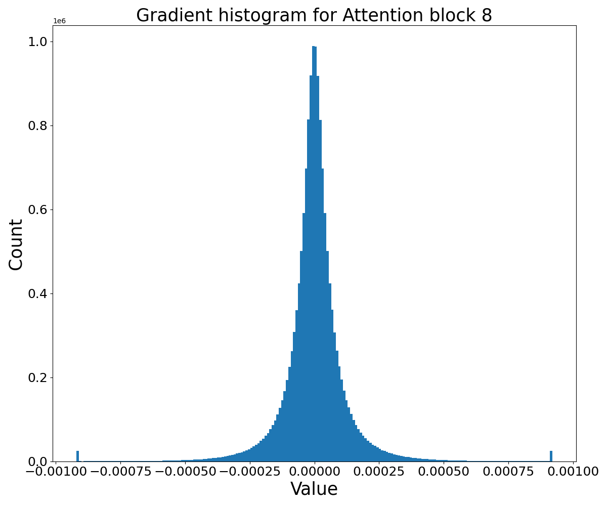
For instance this is the histogram of gradients for GPT2-medium block 10 for the attention QKV weight matrix. We computed the gradient of a single dataset example to prevent averaging between gradients in the batch. In any case, the gradients appear highly Gaussian with 0 mean, but with a few consistent outliers at low or high values. The consistent outliers at 0.0001 and -0.0001 likely reflect the gradient clipping threshold and that in practice without clipping these outliers can be much larger.
Again, this is probably due to CLT-style summation of values in the backward pass. Here, again we can see the challenge of gradient descent and backprop to fight against the information destroying properties of CLT. This is likely a serious source of gradient noise which must be counteracted with large batch sizes.
While this is just one gradient example, we have plotted a great many of them and they almost all follow this pattern.
All Weight Parameters Show The Same Singular Value Pattern (Power Law)
An intriguing pattern emerges when we study the distribution of singular values of weight matrices in transformer models. If we plot the singular value against its rank on a log-log scale, we see a highly consistent pattern of a power-law decay followed by a rapid fall-off at the ‘end’ of the ranks.
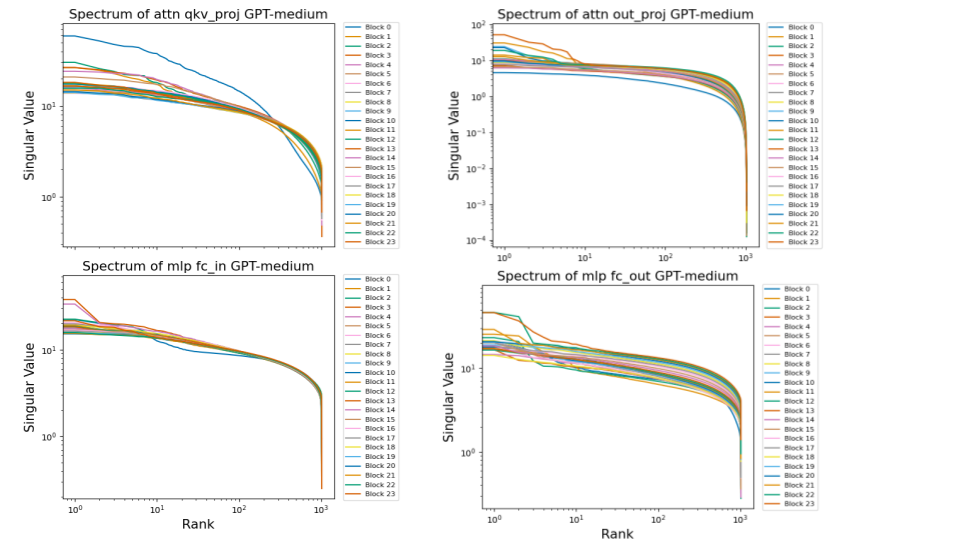
Here we have plotted the spectrum of the weight matrices of all blocks of GPT2-medium. We see that the singular values of the weights of all blocks tend to follow a highly stereotypical power law behaviour with a drop-off at around the same point, suggesting that all of the weight matrices are slightly low rank. Interestingly, most blocks have approximately equal spectra and sometimes there is a clear weight ordering with the singular values either increasing or decreasing with depth.
The first interesting thing is that this spectrum implies that the weight distribution is not as truly Gaussian as it first appears. The spectrum of Gaussian random matrices should follow the Marchenko-Pastur distribution which is very different to the power-law spectrum we observe.
The power law spectrum is highly interesting because it is observed in many real world systems, including in the brain. The power-law spectrum may be related to the expected Zipfian distribution of natural language text but empirically the covariance of the input data follows a different (albeit still power-law) distribution. Power-laws are also implicated in the scaling laws as well as analytical solutions to them which may be connected.
Finally, the rapid fall-off in the singular values implies that the weight matrices are not truly full-rank but have an ‘effective rank’ slightly smaller than the size of all weights. This probably indicates that not all dimensions in weight space are being fully utilized and may also suggest some degree of overparametrization of the model.
Activation Covariances Show The Same Power Law Pattern Of Singular Values
If we measure the covariance matrices of activations in the residual stream across sequences or across multiple batches, we see similar power-law spectra with a clear pattern of increasing singular value spectra in later layers. These plots were generated by computing the covariance matrix between activations in the residual stream over a large amount ~10000 random sequences of the Pile through a pretrained GPT2-small.
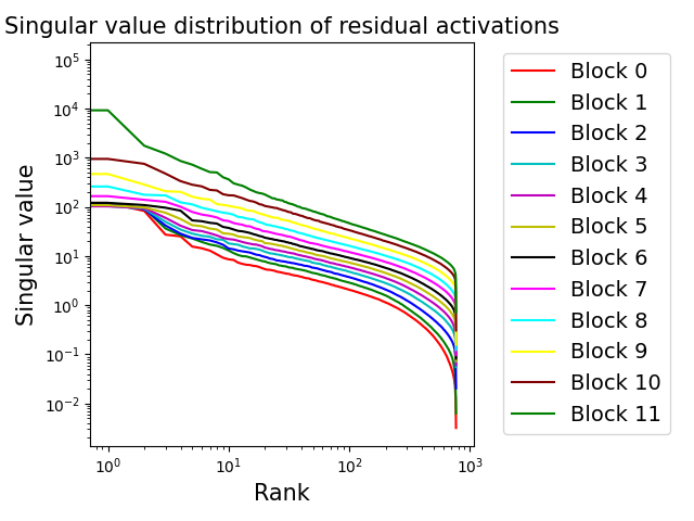
We are still unclear as to the reason for this or what it implies about network processing.
Dataset Covariance Matrix
Ultimately, it appears likely that these power law fits are mimicking the structure of natural text data found on the internet. To test this, we approximated the covariance matrix of the dataset that LMs are trained on. Computing the full covariance matrix over all the data was clearly infeasible, so we instead computed the token-token covariance matrix over a randomly sampled subset of the data that consisted of 100,000 sequences of 1024 tokens from the test-set of the Pile. We then computed the spectrum of this approximately 50k x 50k matrix, which revealed an exceptionally clear power law.
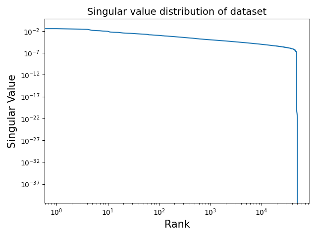
Even when we computed the dataset over 100000 sequences, it appears that there is some redundancy in the token matrix resulting in the token-token covariances being low rank (explaining the extremely sharp dropoff). This is likely due to lacking single examples of the conjunction of exceptionally rare tokens.
It seems likely, then, that the spectrum of the weights and activations in the network tend to mimic that of the dataset it was trained upon. Such mimicry of the spectrum of the data is potentially the optimal approach in reconstruction tasks like the next-token-prediction the LLM is trained upon. This also supports the scaling law argument of Maloney et al(2022) which argues that power-law scaling laws arise due to needing to model power-laws in the spectrum of natural data.
19 comments
Comments sorted by top scores.
comment by Fabien Roger (Fabien) · 2023-01-04T17:45:59.110Z · LW(p) · GW(p)
I'm surprised you put the emphasis on how Gaussian your curves are, while your curves are much less Gaussian that you would naively expect if you agreed with the "LLM are a bunch of small independent heuristic" argument.
Even ignoring outliers, some of your distributions don't look like Gaussian distributions to me. In Geogebra, exponential decays fit well, Gaussians don't.
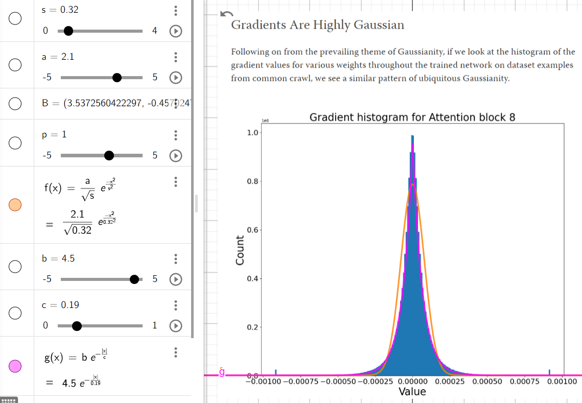
I think your headlines are misleading, and that you're providing evidence against "LLM are a bunch of small independent heuristic".
Replies from: StellaAthena, GuySrinivasan↑ comment by StellaAthena · 2023-01-04T17:54:11.132Z · LW(p) · GW(p)
This is very interesting. The OP doesn’t contain any specific evidence of Gaussianness, so it would be helpful if they could provide an elaboration of what evidence lead them to conclude these are Gaussian.
↑ comment by SarahNibs (GuySrinivasan) · 2023-01-04T18:39:53.032Z · LW(p) · GW(p)
When investigating distributions from a completely different source, I thought for a while
- these are all pretty gaussian! except for the bits on the right, and I know where those come from
then recognized that their tails were wider and thought
- maybe they're ... student-t or something? [confused]
and eventually realized
- oh, of course, this is a mixture of lots of gaussians; each natural class induces a gaussian in the limit, but this distribution represents a whole slew of natural classes, and most of their means are quite similar, so yeah, it's gonna look like a fatter-tailed gaussian with some "outliers"
and I think this probably happens quite a lot, because while CLT ==> gaussian, nature rarely says "here's exactly one type of object!"
Replies from: Fabien↑ comment by Fabien Roger (Fabien) · 2023-01-04T18:45:56.613Z · LW(p) · GW(p)
If you sum enough Gaussians you can get close to any distribution you want. I'm not sure what the information behind "it's Gaussian" in this context. (It clearly doesn't look like a mixture of a few Gaussians...)
Replies from: GuySrinivasan↑ comment by SarahNibs (GuySrinivasan) · 2023-01-04T19:13:20.920Z · LW(p) · GW(p)
It clearly doesn't look like a mixture of a few Gaussians
It does to me. If their means are close enough compared to their variances, it'll look like a unimodal distribution. For a good example, a student t distribution is a mixture of gaussians with the same mean and variances differing in a certain way, and it looks exactly like these images.
See the first image here: https://en.m.wikipedia.org/wiki/Student's_t-distribution
comment by ryan_greenblatt · 2023-01-04T20:34:25.319Z · LW(p) · GW(p)
In prior work I've done, I've found that activations have tails between and (typically closer to ). As such, they're probably better modeled as logistic distributions.
That said, different directions in the residual stream have quite different distributions. This depends considerably on how you select directions - I imagine random directions are more gaussian due to CLT. (Note that averaging together heavier tailed distributions takes a very long time to be become gaussian.) But, if you look at (e.g.) the directions selected by neurons optimized for sparsity, I've commonly observed bimodal distributions, heavy skew, etc. My low confidence guess is that this is primarily because various facts about language have these properties and exhibiting this structure in the model is an efficient way to capture this.
This is a broadly similar point to @Fabien Roger.
Replies from: christopher-olah, StellaAthena↑ comment by Christopher Olah (christopher-olah) · 2023-01-05T04:25:29.993Z · LW(p) · GW(p)
See also the Curve Detectors paper for a very narrow example of this (https://distill.pub/2020/circuits/curve-detectors/#dataset-analysis -- a straight line on a log prob plot indicates exponential tails).
I believe the phenomena of neurons often having activation distributions with exponential tails was first informally observed by Brice Menard.
↑ comment by StellaAthena · 2023-01-04T21:03:59.096Z · LW(p) · GW(p)
Do you have a reference to the work you’re talking about? I’m doing some stuff involving fitting curves to activation tails currently.
Replies from: ryan_greenblatt↑ comment by ryan_greenblatt · 2023-01-04T21:26:07.394Z · LW(p) · GW(p)
Unpublished and not written up. Sorry.
comment by StellaAthena · 2023-01-04T15:13:10.667Z · LW(p) · GW(p)
I’m not sure when you developed this work, but the LLM.int8 paper identifies outliers as an essential factor in achieving performance for models larger than 2.7B parameters (see Fig. 1 and Fig. 3 especially). There’s also some follow-up work here and here. Very curiously, the GLM-130B paper reports that they don’t see outlier features at all, or the negative effects of their lack of impact.
I’ve spoken with Tim (LLM.int8 lead author) about this a bit and some people in EleutherAI, and I’m wondering if there’s some kind of explicit or implicit regularizing effect in the GLM model that prevents it from learning outlier features. If this is the case, one might expect to find different patterns in outliers in models with sufficiently different architecture, perhaps GPT-2 vs Pythia vs GLM vs T5
comment by nostalgebraist · 2023-01-05T03:44:31.759Z · LW(p) · GW(p)
This CLT mixing effect might be expected to destroy information in the representations, as occurs in the NTK limit of infinite width where the CLT becomes infinitely strong and no information can be propagated between layers. It is not clear how the network preserves specific and detailed information in its activations despite near-Gaussian mixing.
Have you looked at Roberts and Yaida's Principles of Deep Learning Theory?
They develop a first-order perturbative correction to NTK, where the perturbative parameter is depth-to-width ratio of the network. The resulting distributions are "nearly Gaussian," with a non-Gaussian correction controlled by the depth-to-width ratio.
Roughly, the authors claim that this regime -- where the O(depth/width) correction to NTK is important but higher-order corrections can be neglected -- is not only tractable, but also where real NNs operate. They make a number of claims about why you'd want the depth-to-width ratio to be small but nonzero, such as
- If the ratio is zero, there's no feature learning (NTK). But feature learning does occur in the first-order (small but nonzero) theory, so maybe that's "enough."
- As the ratio grows larger, vanishing/exploding activations and gradients become more and more likely, when considered across different initialization draws, test inputs, etc. -- even if you pick an initialization scheme that is well behaved on average.
- They make an argument connecting this ratio to the bias-variance tradeoff, where overly deep/narrow networks become overly high-variance. (IIUC this is the extension of "across initialization draws, test inputs, etc." in the previous point to "...across draws of the training data.")
- They also have another argument involving mutual information ... suffice it to say they have a lot of these arguments :)
(I have only skimmed the book and can't really claim to understand it, so I'm mostly bringing it up because it sounds like you'd find it relevant.)
Replies from: danroberts↑ comment by danroberts · 2023-01-07T19:10:45.945Z · LW(p) · GW(p)
Thanks for your summary of the book!
I think that the post and analysis is some evidence that it might perhaps be tractable to apply tools from the book directly to transformer architectures and LLMs.
comment by Mateusz Bagiński (mateusz-baginski) · 2023-01-05T06:46:22.225Z · LW(p) · GW(p)
It would be interesting to see how these change throughout training. AFAIK GPT-2s do not have saved checkpoints, but eg Pythia does and has an even broader range of parameter sizes than GPT-2s.
comment by Charles Martin (charles-martin) · 2023-01-05T03:20:40.375Z · LW(p) · GW(p)
The PowerLaw behavior has been noted for some time. See https://weightwatcher.ai and the publications in JMLR and Nature Communications.
comment by ObserverSuns · 2023-01-05T01:46:01.401Z · LW(p) · GW(p)
Would it be possible for you to share any of the code you used to obtain these results? This post has inspired me to run some follow-up analyses of my own along similar lines, and having access to this code as a starting point would make that somewhat easier.
Replies from: beren↑ comment by beren · 2023-01-05T15:29:40.071Z · LW(p) · GW(p)
Unfortunately our code is tied too closely to our internal infrastructure for it to be worth disentangling for this post. I am considering putting together a repo containing all the plots we made though, since in the post we only publish a few exemplars and ask people to trust that the rest look similar. Most of the experiments are fairly simple and involves just gathering activations or weight data and plotting them.
comment by TurnTrout · 2023-05-03T00:46:08.854Z · LW(p) · GW(p)
Some hypotheses about such functions could be that the outliers perform some kind of large-scale bias or normalization role, that they are ‘empty’ dimensions where attention or MLPs can write various scratch or garbage values, or that they somehow play important roles in the computation of the network.
If the outliers were garbage values, wouldn't that predict that zero ablation doesn't increase loss much?
comment by Review Bot · 2024-08-09T19:57:48.905Z · LW(p) · GW(p)
The LessWrong Review [? · GW] runs every year to select the posts that have most stood the test of time. This post is not yet eligible for review, but will be at the end of 2024. The top fifty or so posts are featured prominently on the site throughout the year.
Hopefully, the review is better than karma at judging enduring value. If we have accurate prediction markets on the review results, maybe we can have better incentives on LessWrong today. Will this post make the top fifty?
comment by cherrvak · 2023-02-23T19:58:58.846Z · LW(p) · GW(p)
It is possible that the outlier dimensions are related to the LayerNorms since the layernorm gain and bias parameters often also have outlier dimensions and depart quite strongly from Gaussian statistics.
This reminds me of a LessWrong comment [LW(p) · GW(p)] that I saw a few months ago:
I think at least some GPT2 models have a really high-magnitude direction in their residual stream that might be used to preserve some scale information after LayerNorm.