Taking features out of superposition with sparse autoencoders more quickly with informed initialization

post by Pierre Peigné (pierre-peigne) · 2023-09-23T16:21:42.799Z · LW · GW · 8 comments

Contents

  0 - Context
        The aim of this project was to reduce the compute required to train those sparse autoencoders by experimenting with better initialization schemes.
    The original training process
    The metric
  I - Initializing the dictionary with input data
      Average speed to high MMCS thresholds
  II - Collecting rare features for initialization
  III - Conclusion and future work
None
8 comments

This work was produced as part of the SERI MATS 3.0 Cohort under the supervision of Lee Sharkey.

Many thanks to Lee Sharkey for his advice and suggestions.

TL;DR: it is possible to speed up the extraction of superposed features using sparse autoencoders by using informed initialization of the sparse dictionary. Evaluated on toy data, the informed initialization scheme results are the following:

• Immediate MMCS ~ 0.65 (MMCS < 30% at start with the original orthogonal initialization)
•  Up to ~10% speedup to reach 0.99 MMCS of the superposed feature with some initialization methods relying on collecting rare features.

The main ideas: 

1. The data contains the (sparsely activating) true features, which can be used to initialize the dictionary
2. However, the rare features are “hard to reach” in the input data. To get a good recovery we want to make sure the rare features are represented in the initialization sample. 

0 - Context

Previous work has investigated how to take superposed features out of superposition in toy data [AF · GW]. However, the current approach based on sparse autoencoders is relatively compute intensive, making the possibility of recovering monosemantic representations of large models computationally challenging.

The aim of this project was to reduce the compute required to train those sparse autoencoders by experimenting with better initialization schemes.

The original training process

To take features out of superposition using sparse autoencoders, we train an autoencoder with an L1 penalty on its hidden layer activation. In order to fit all (or at least the maximum of) superposed features in a monosemantic manner, the decoder dimensions must be larger or equal to the total number of ground truth (superposed) features. 

Current initialization of the decoder relies on orthogonal initialization (Hu et al. 2020).

The metric

I used the same metric as in the original work: the Mean Max Cosine Similarity [AF · GW]. 

This metric is supposed to capture how well the ground features are recovered by the sparse dictionary. For instance an MMCS of 0.65 means that, on average, each ground truth feature has, on average, a cosine similarity of 0.65 with the most similar learned feature.

I - Initializing the dictionary with input data

The idea is that even though the ground truth features are superposed, the data still contain useful information about the structure of the ground truth features. Therefore, if we use data samples as initialization vectors, the training of the sparse dictionary does start from scratch but leverages the structure of the input data to reconstruct the original features.

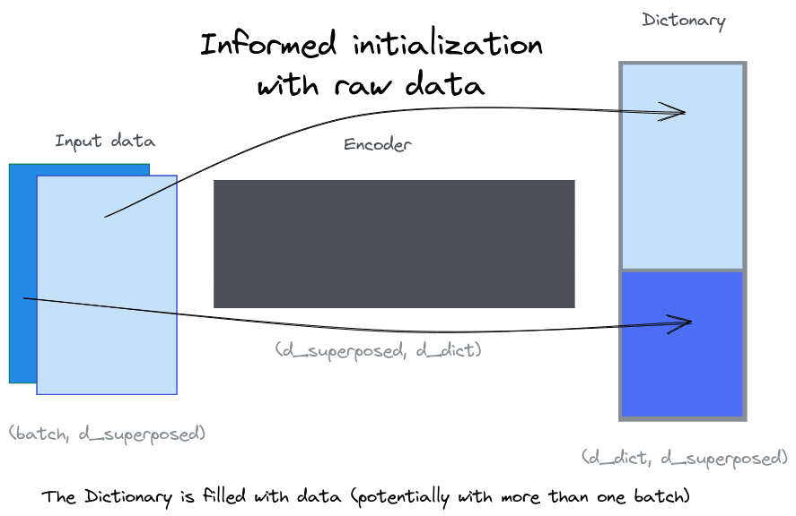
I compared four methods of initialization: two conventional methods (Xavier and orthogonal init) and two based on the input data (initialization using SVD of a random sample of the data and initialization using a sample of the raw data directly). 

Initialization using input data:

1. Raw data: we take a sample of the data and use it as initialization weights for the dictionary.
2. SVD data: we take a sample of the data and apply Singular Value Decomposition to it. We then use the results of the SVD to initialize the dictionary with the $U$matrix^[1]. 

These four methods were tested in three different scenarios: 128/256, 128/512 and 128/1024. 
In each scenario, the first number refers to the dimension of the vector where the ground truth features are compressed into, and the second refers to the original dimension of the ground truth features. For instance in 128/256, the 256-dimensional ground truth features are compressed into a 128-dimensional space. In each case, the dictionary size was the same as the number of ground truth features. 

Average speed to high MMCS thresholds

The following graphs show the MMCS by time step given different initialization schemes. Ranges where 0.95, 0.98 and 0.99 MMCS thresholds were reached are highlighted.

The training was stopped once 0.99 MMCS was achieved or after a given number of steps (140 for 128/256 and 128/512, and 400 for 128/1024). 

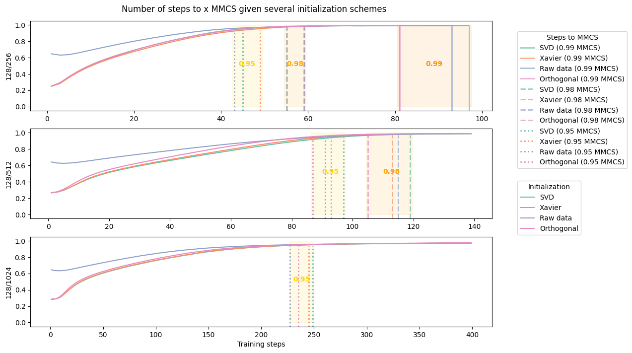
There are two observations to be made from this graph: 

1. Raw data init does provide a much better start than orthogonal initialization: the MMCS is immediately above 0.60.
2. But, it fails to reach high MMCS scores more quickly than orthogonal initialization. Even if raw data succeed to reach 0.95 MMCS more quickly on average for the 128/256 and 128/1024 scenarios, it is already outperformed by orthogonal init in the 128/512 one. Then, once the 0.95 threshold passed, orthogonal initialization always beat raw data in terms of speed.

We hypothesize that reaching 0.99 MMCS requires recovering the rare features which are either not present in the raw data sample or hidden behind the most common ones.

II - Collecting rare features for initialization

Our hypothesis is that rare features are slower to learn than the most common ones.  So we want to find a way to collect some of the rare features in order to use them as initialization parameters for our sparse dictionary.
 

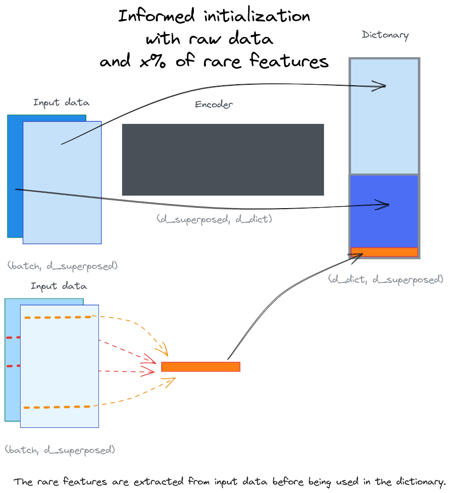
Hence we devised two main approaches to try to get them: 

1. Subtracting the most common feature from a random sample hoping that the remaining will represent some rare feature. I tested two techniques: average and centroid based. 
   1. Average based technique: this is the most naïve and raw approach. It consists in subtracting the average value of an entire batch from one randomly selected element and then using the remaining as “rare feature vectors”.
   2. Centroid based technique: this is a (slightly) finer approach where we clusterize the data and then for each cluster we collect a random sample and subtract it the value of its cluster’s centroid. I performed clustering using MiniBatchKMeans with a number of clusters equal to the number of “rare feature” vectors we were looking for. 
2. Detecting outliers and collecting them: we expect that outliers would correspond to samples having explicit rare features (i.e. not hidden by some most common ones). I used LocalOutlierFactor with a n_neighbors parameter of 250.

The following graphs show the number of steps to 0.99 MMCS convergence (for the three methods applied to the 128/256 and 128/512 scenarios^[2]). The results were evaluated for a range of “rare features” ratio between 0.1% and 20%. 

Caution: those results are a bit weird and not very conclusive. I suggest the reader to stay cautious about not taking too much out of them.

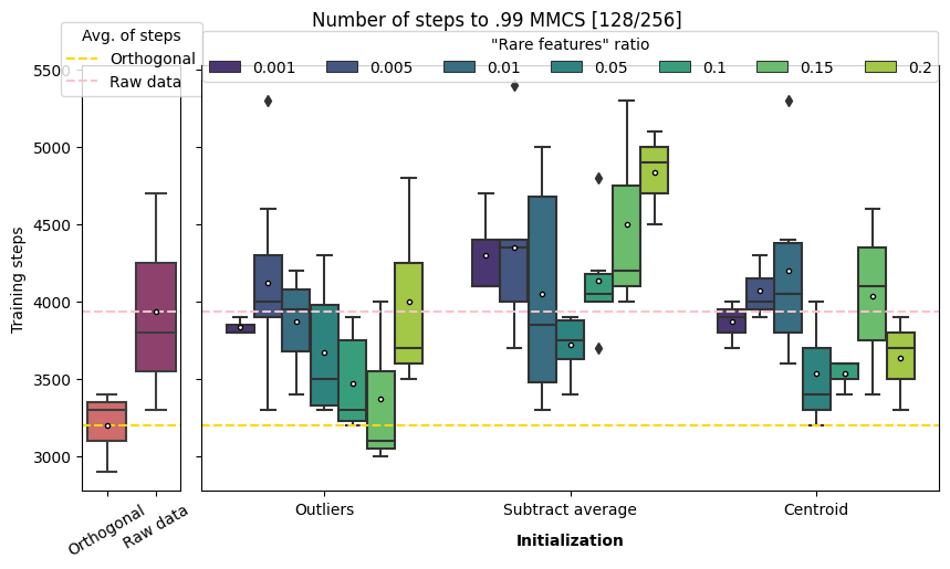
On average outliers detection with a “rare features” ratio between 1 and 15% is faster than raw data initialization. 

Centroid works better for 5, 10 and 20% but not 15%. This weird result could be an artifact of the method: the number of clusters is arbitrarily determined by the number of rare features vectors we want to collect. Therefore, it could be possible for the number of clusters used in the MiniBatchKMeans to be different from the number of meaningful clusters in the true features. By sampling centroid from “un-natural” clusters, we are not collecting meaningful features to be subtracted from samples to uncover rare features.

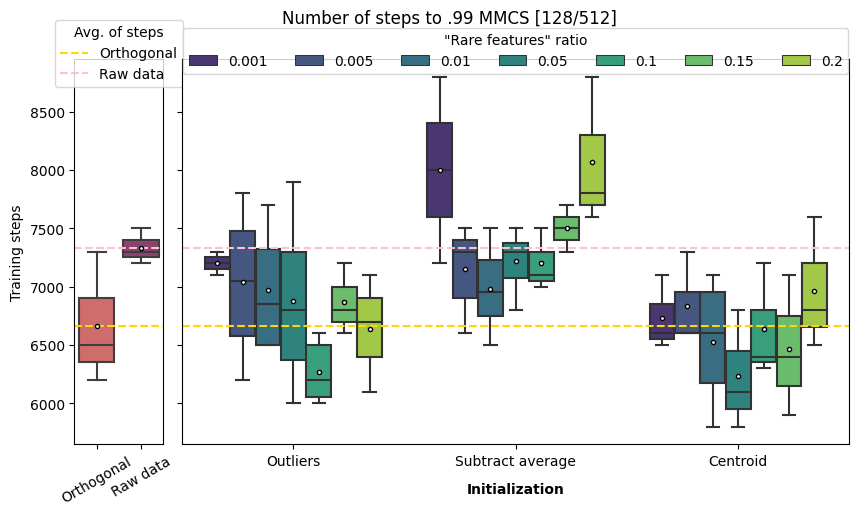
On average centroid based and outlier detection always outperform raw data initialization for the scenario 128/512. Even the very naive approach of subtracting average performs better with a rare features ratio between 0.5 and 10%. 

Outlier detection of 10% and 20% (but weirdly not 15%) beat the orthogonal initialization while centroid based approach is quicker for a range of parameters between 1% and 15%, reaching a ~10% speedup at 5% of rare features.

III - Conclusion and future work

These results are very limited in terms of scope (only two scenarios were tested entirely), data (the experiments used synthetic ones), “rare features collection” methods, and hyperparameters. My main bottleneck was the training time: sparse dictionary learning is a time consuming task (that's the point of this entire project) and therefore I was limited in my ability to iterate. 

It seems plausible that more speedup could be reached by experimenting in that direction but I am uncertain about the extent of what is reachable using informed initialization. 

Here are some ways this work could be extended:

1. Finding optimal hyperparameters for the outlier detection and/or the centroid approach.
2. Testing other outlier detection and/or clustering techniques.
3. Testing for higher superposition ratio (more features in the same embedding space).
4. Testing the results with dictionary size different from the true feature dimensions.
5. Testing this approach on real data (i.e. real activation of a transformer model).

If you are interested in working on this topic, please reach out!

1. ^{^}

    Singular Value Decomposition (SVD) decomposes a matrix $M$ of shape $(m\times m)$ into three matrices: $M=U_{(m\times m)}{\Sigma }_{(m\times n)}{V}_{(n\times n)}^T$, where $U$ contains left singular vectors of shape (m x m). Each column of $U$represents a basis vector in the original data space, and these vectors encode salient features of the data, with the leftmost columns corresponding to the most significant features, as determined by the associated singular values in $\Sigma$.

2. ^{^}

    The training time for the 128/1024 scenarios being too long, I did not perform this evaluation for this one. I’d be happy to see the results of this if anyone wants to replicate those experiments. 

8 comments

Comments sorted by top scores.