[Interim research report] Taking features out of superposition with sparse autoencoders

post by Lee Sharkey (Lee_Sharkey), Dan Braun (dan-braun-1), beren · 2022-12-13T15:41:48.685Z · LW · GW · 23 comments

Contents

  Introduction
  Methods
    Toy dataset generation
    Sparse autoencoder architecture and training
    Measuring ground truth feature recovery with Mean Max Cosine Similarity (MMCS)
    Small transformer trained on natural language data
  Experimental results
    The L1 penalty coefficient needs to be just right
    We need more learned features than ground truth features
    Complication: Optimal L1 penalty coefficient interacts with optimal dictionary size
    Finding the right hyperparameters without access to the ground truth
      Method 1: The presence of dead neurons
      Method 2: Loss stickiness
      Method 3: Mean max cosine similarity between a dictionary and those larger than it
  Identifying the overcomplete feature basis used in a language model
    Dead neurons
    Loss stickiness
    Mean max cosine similarity between a dictionary and those larger than it
  Conclusion
  Appendix
    Denoising autoencoders (with the right amount of noise) are sparse autoencoders that recover ground truth features
    Heatmaps for L1 penalty coefficient vs Dictionary size for all layers
      Dead neurons
      Loss stickiness
      Mean max cosine similarity between a dictionary and those larger than it
None
24 comments

We're thankful for helpful comments from Trenton Bricken, Eric Winsor, Noa Nabeshima, and Sid Black. 

This post is part of the work done at Conjecture.
 

TL;DR: Recent results from Anthropic suggest that neural networks represent features in superposition. This motivates the search for a method that can identify those features. Here, we construct a toy dataset of neural activations and see if we can recover the known ground truth features using sparse coding. We show that, contrary to some initial expectations, it turns out that an extremely simple method – training a single layer autoencoder to reconstruct neural activations with an L1 penalty on hidden activations – doesn’t just identify features that minimize the loss, but actually recovers the ground truth features that generated the data. We’re sharing these observations quickly so that others can begin to extract the features used by neural networks as early as possible. We also share some incomplete observations of what happens when we apply this method to a small language model and our reflections on further research directions. 
 

This post is not intended to be a polished research product. It’s a set of preliminary and incomplete results that we’d like to share early in case it benefits the broader mechanistic interpretability research community. 

Introduction

Features in a neural network are represented in high dimensional neural activations. Recent work from Anthropic has demonstrated that neural networks probably use a phenomenon called superposition to represent more features than available dimensions. Superposition is a challenge for mechanistic interpretability because it leads to polysemanticity, which prevents us from telling simple, human-understandable stories about how individual representations in neural networks relate to each other. Superposition also introduces another, more practical problem: Many of the best known feature extraction methods are dimensionality reduction techniques that find at most $N$ directions in an $N$ dimensional space. But we need a method that finds more than $N$ features in superposition (i.e. an ‘overcomplete’ set of features). If we could develop a method that decomposes a neural network’s activations into its component features, we would essentially be taking features out of superposition, thus resolving the problems that superposition causes for interpretability. 

Superposition is possible because not all features are active at any one time. In fact, we expect that only a few features are active at any one time; in other words, feature activations may often be sparse. The sparsity of feature activations suggests that a set of methods called sparse coding or sparse dictionary learning (Olshausen & Field, 1996; Chen et al. 2001; Donoho et al. 2003) may offer a way to identify the underlying features used by networks. 

Although there are many different sparse coding algorithms, one of the simplest and most scalable methods is a single-layer feedforward autoencoder with sparsity (L1 norm) regularization on its hidden activations. When training a sparse autoencoder to reconstruct toy data – a ‘fake’ dataset of neural signals where we generate the data from sparse linear combinations of known ground truth feature directions – the results we present here indicate (to our slight surprise) that the decoder weights learned by a sparse autoencoder actually approximate the underlying ground truth features used to generate the data. It wasn’t a priori obvious to us that it would do this, nor to a couple of other researchers whom we’ve talked to who were working on this problem. To our intuitions at least, it might plausibly have learned features that performed well in terms of reconstruction loss but poorly in terms of ‘recovering the ground truth features’. Our intuitions notwithstanding, there is a (somewhat involved) proof that linear combinations of ground truth features can be recovered by L1 minimization in Chapter 3 of High-dimensional data analysis with Low Dimensional Models by Wright & Ma. Some recent work in the disentangled representations literature independently demonstrated that autoencoders recover ground truth features under certain constraints, including sparsity and non-negativity (both present in our experiments) (Whittington et al., 2022). 

After demonstrating that feedforward sparse autoencoders can recover the true data generating features, we apply the method to the MLP activations of a small ($31$M parameters) language model that we trained ourselves. We explore three approaches that might let us identify whether we’ve actually found the ground truth features even though we don’t have direct access to them. The results from the language model MLPs are sufficiently different from the toy data that they demand further, clarifying experiments. Specifically, we plan to explore what changes to the toy data are required to make the toy results look more like the results from the MLPs, which should help us identify whether we’ve recovered the ground truth features used by networks. However, to speed up research dissemination in the mechanistic interpretability community, we are releasing our toy-model results here so that others can build upon our efforts in parallel if they’re interested in doing so.

Methods

Toy dataset generation

We wanted to create toy data that resemble neural data but where we have access to the ground truth components that compose the data. 

First, we defined a set of ground truth features by uniformly sampling $G=512$ independent samples from a $h$-dimensional sphere. This creates a $h\times G$ matrix of ground truth features $F$ that we want to recover using sparse coding. In our toy data experiments $h=256$. In the language model experiments $h$ is the dimension of the hidden layer of the MLP (in our language model, $4\times d_{model}=1024$). In the toy data experiments, $G$ is therefore $2h$, and thus defines an overcomplete set of features since there are twice as many features as dimensions. We don't know how many features the language model uses, but we expect our empirical value of $G$ to be larger than $h$. 

After defining the ground truth features, we then constructed sparse ground truth feature coefficients by (1) sampling from a $G$-dimensional binary random variable that takes $0$ with high probability and $1$ with low probability such that on average $5$ out of $G$ ground truth features are active at a time, and (2) scaling those sparse binary vectors by multiplying them with a $G$-dimensional vector where each element is sampled from a uniform distribution between $0$ and $1$ to obtain an ‘activation’ for that feature. To better simulate the expected statistical properties of features in real neural data, we sampled a binary random vector such that some features were more likely to be active than other features and there were correlations between feature activations using the following procedure:

• To create correlations between features (i.e. when one feature is active, another is more likely to be active), we need to create correlations between sparse activations of the $G$-dimensional binary random variable. To do this, we created a random covariance matrix for a multivariate normal distribution with zero mean. We took a single sample from a correlated multivariate normal distribution and, for each dimension of that sample, found where that sample lay on the standard normal cumulative distribution function. This gets us a vector taking values in $(0,1)$ that shares a correlation structure that depends on the random, fixed covariance matrix that we used for the multivariate normal distribution. 
• To make some features have greater frequency than others, we modified the above so that the probability of the $G$-dimensional random variable exponentially decayed with the feature’s index (i.e. the probability of the $g^{\text{th}}$ feature is $p_g=(p_g^{\prime }{)}^{g\lambda }$ where $\lambda =0.99$ and $p_g^{\prime }$ is the correlated feature probability defined using the above procedure). 
• After exponentially decaying the correlated feature probabilities, we rescaled all probabilities using the following method: first, we calculated the mean probability of all features. Then, we calculated the ratio of the number of ground truth features that are active at a time ($5$ out of $G$ in this case) to the mean probability. Finally, we multiplied each probability by this ratio to rescale them, ensuring that on average $5$ out of $G$ ground truth features are active at a time. 

We can use the correlated, decayed, rescaled vector to parameterize a vector of Bernoulli random variables, which we use as the $G$-dimensional binary random variable in step (1) for defining sparse ground truth feature coefficients. To create our dataset, we use the sparse coefficients to linearly combine a sparse selection of the ground truth features. 

Sparse autoencoder architecture and training

We trained an autoencoder to reconstruct the toy data (or the MLP activations in the language model experiments). The inputs to our autoencoder(s) were $h$-dimensional vectors $x\in X$; these are the toy data (described above) in the toy data experiments and MLP activations in the language model experiments. 

Our autoencoder(s) consist of a linear layer (a $J\times h$ weight matrix $W_e$ with a $J$-dimensional bias vector $b_e$) followed by a ReLU activation. The output of the encoder is therefore $c=\text{ReLU}(W_{e}x+b_e)$, a $J$-dimensional vector of dictionary element coefficients. The encoder is followed by a learned dictionary of features, $D$, which is a $h\times J$ decoder matrix (with no bias) whose columns (the learned features) are constrained to have unit norm on the forward pass. The learned dictionary uses orthogonal initialization (Hu et al. 2020). Ultimately, we want the learned dictionary elements ($\left\{D_j\right\}$ to recover the ground truth feature directions used to generate the dataset ($\left\{F_g\right\}$) without incentivising their recovery directly in the loss function. During training, we impose an $L_1$ regularization penalty on the dictionary element coefficients, thus encouraging the network to activate only a small number of the dictionary elements at a time. Overall, the loss function is therefore $L=L_{\text{reconstruction}}+L_{L_1}=\frac{1}{h}||x-Dc|{|}^2+\frac{1}{J}\alpha \ast |c|$. We used the Adam optimizer in all experiments (learning rate $0.001$, batch size $256$). 

In the toy data experiments, unless otherwise stated, the dictionary size was fixed to be the same as the number of ground truth elements, i.e. $J=G=2\times h=512$. In later experiments we varied the dictionary size so that $J$ doesn’t necessarily equal $G$).

Measuring ground truth feature recovery with Mean Max Cosine Similarity (MMCS)

To measure how well the learned dictionary recovered the ground truth features, we took the ‘mean max cosine similarity’ (MMCS) between the ground truth features and the learned dictionary. 

Formally, the mean max cosine similarity between the learned dictionary $D$ and the ground truth features $F$ is:

$MMCS=\frac{1}{G}{\sum }_{g=1}^G{max}_j\text{CosineSim}(D_j,F_g).$

Intuitively, to calculate the MMCS, we first calculate the cosine similarity between all pairs of dictionary elements in the learned and ground truth dictionaries. Then, for every ground truth dictionary element, we find the learned dictionary element with the maximum cosine similarity. Then we take the mean of those maxima. This finds the learned feature that is most similar to each ground truth feature and measures how well the ground truth was recovered. The reason we need to do this is that even if the autoencoder perfectly reconstructed the ground truth, the set of learned dictionary elements may still be a permutation of the set of ground truth features, so we need to find the dictionary element that best matches each ground truth feature. We can measure the mean max cosine similarity even when the number of ground truth and learned dictionary elements are different because we ignore the learned dictionary elements that aren’t among the maximally similar elements to one of the ground truth features. 

In language model experiments, we don’t have access to the ground truth features. But we nevertheless make use of the MMCS by comparing learned dictionaries of different sizes (we justify why in section `Method 3: Mean max cosine similarity between a dictionary and those larger than it`). In that case, we simply replace $F$ in the above equations with the smaller of the two dictionaries being compared. 

Small transformer trained on natural language data

Although the first half of this post discusses results that apply autoencoders to toy data, later experiments use real data collected from a small ($31$ million parameter, $d_{model}=256$) six-layer transformer. The transformer uses a standard GPT2 decoder-only architecture, a GELU activation function, four attention heads, a vocabulary size of $50304$, and learned positional embeddings. It was trained using the Adam optimizer (learning rate annealed from $0.0012$ to $0.00012$; cosine annealing schedule with warmup on 1% of the data; with weight decay $0.1$) with a batch size of 256 on the Wikipedia subset of the Pile dataset ($30B$ tokens) (Gao et al., 2021), achieving a cross entropy loss of $3.074$ on the training data (perplexity per token: $20.906$).

Experimental results

The L1 penalty coefficient needs to be just right

One of the main hyperparameters involved in sparse autoencoders is the L1 penalty coefficient. If the L1 penalty coefficient is too high, then the autoencoder will be too sparse (i.e. too few dictionary elements will activate); if the penalty is too low, then the autoencoder will not be sparse enough (i.e. too many elements will activate).

When we train sparse autoencoders with different L1 penalties, we see a ‘Goldilocks zone’ in which the autoencoder recovers the ground truth features:

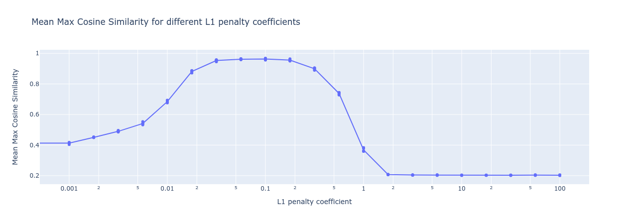
The range of acceptable L1 penalties is wide, ranging over almost an order of magnitude, from around $0.03$ to around $0.3$. But when we train sparse autoencoders on real data, we won’t be able to measure the mean max cosine similarity with the ground truth features like we did above. We’re going to need a way to identify when we’ve got the right L1 penalty coefficient. 

We need more learned features than ground truth features

In the above experiments, we assumed we knew the exact number of ground truth features and accordingly set the number of learned dictionary elements to be exactly equal. But when we train sparse autoencoders on real neural data, we won’t know how many features are represented in the activations. We’re going to need a way to figure out when we’ve got the right number of learnable dictionary elements in our autoencoder.

Fortunately, the autoencoder appears robust to overparameterization – it seems like we can simply increase the number of features in our learned dictionary (within reason) and it continues to reconstruct the correct features even though it has many ‘redundant’ features. This increases our confidence that we can recover ground truth features as long as we make our dictionary big enough .

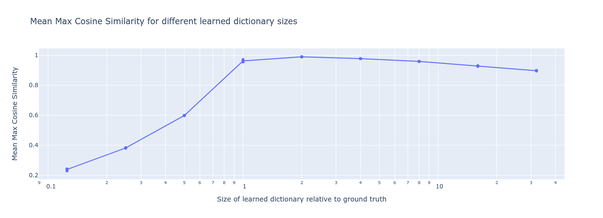
We see that we can almost completely recover the true ground features using dictionaries that are between 1-8$\times$ the size of the ground truth dictionary, with the MMCS only slowly decreasing as we continue increasing the learned dictionary size. However, increasing the dictionary size comes with a computational cost. In practice, we therefore can’t simply use arbitrarily large dictionaries in order to be sure that we have enough learnable features. We will need a method to identify when to stop increasing the size of our learnable dictionary in order not to waste computation.

Complication: Optimal L1 penalty coefficient interacts with optimal dictionary size

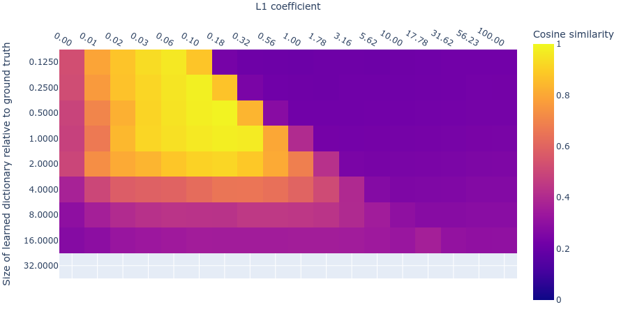
Notice in figure 2 that larger learned dictionaries have slightly lower MMCS than the learned dictionaries that are the right size. The decreasing MMCS may be due to an interaction between the optimal L1 penalty coefficient and the optimal dictionary size. Below we plot the mean max cosine similarity for different dictionary sizes and L1 parameters. Indeed, it turns out that you need large L1 penalties for larger dictionaries. 

This complicates our search for the optimal hyperparameters because the hyperparameters are not independent and so we can’t search over hyperparameters one at a time; we have to search over both hyperparameters simultaneously. Nevertheless, as long as we have a reasonably large dictionary size, there is a large range of acceptable L1 penalty coefficients.

Finding the right hyperparameters without access to the ground truth

In all the above experiments, we had access to the ground truth features. This lets us calculate the mean max cosine similarity between the learned features and the ground truth features and thus identify a set of optimal L1 penalty coefficients and dictionary sizes. Notably, a dictionary size of $1.0$ (relative to the number of ground truth features) and an L1 penalty coefficient of roughly $0.03$ to $0.3$ are optimal, but we’d also accept larger dictionaries and correspondingly larger L1 penalties. Remember these optimal hyperparameters (Dict Size 1.0; L1 coeff 0.03 to 0.3); we’ll want to see if our methods can recover them. 

Here we develop three ways to estimate when we’ve got the right hyperparams for our sparse autoencoder without access to the ground truth features. We reasoned that, if the properties of real neural data differs from our toy data in some meaningful way, having multiple methods to estimate the degree of recovery of ground truth features will let us cross reference the optimal hyperparameters suggested by each method; if different data properties cause one method to be wrong, then hopefully the others might nevertheless let us find the right ones. The methods are:

1. The presence of dead neurons
2. Loss stickiness
3. Mean max cosine similarity between a dictionary and those larger than it

Method 1: The presence of dead neurons

One of the classic problems with ReLU activations is that it was believed to lead to ‘dead neurons’, where a neuron might reach a state where no input on the training distribution activates it. Since its activation is therefore always zero, no gradients can backpropagate through it, and hence it will always remain ‘dead’.

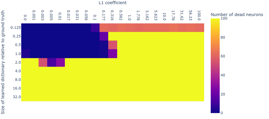
We found that, at least for our toy data, dead neurons almost never arose when the number of learnable features was fewer than or equal to the number of ground truth features. We counted a dead neuron as one that didn’t activate (i.e. its post-ReLU value was $0$) in the last $T$ minibatches (where $T$ was $500$ in toy data experiments and $3000$ in language model experiments). However, as we increase both L1 penalty coefficient and dictionary size, dead neurons begin to appear when either the L1 penalty coefficient is too high or the dictionary size is too big. Notice that the largest dictionary with the largest L1 penalty coefficient that has no dead neurons (i.e. Dict Size $1.0$; L1 coeff $0.177$) lies perfectly within our desired hyperparameter range (Dict Size $1.0$; L1 coeff $0.03$-$0.3$) where the MMCS with the ground truth is highest. This indicates that we might be able to use dead neurons to identify the hyperparameters for which ground truth feature recovery is optimal.

Method 2: Loss stickiness

It’s important to appreciate that we can’t simply use the reconstruction loss to identify whether our sparse autoencoder has recovered the ground truth features. The autoencoders can get low reconstruction loss but poor ground truth feature-recovery when the L1 penalty coefficient is too low. 

An interesting pattern in the loss nevertheless emerges when we plot the loss on a log scale. We see that, as we increase the L1 penalty coefficient, there is a basin where the reconstruction loss remains roughly constant even though L1 is increasing. When the L1 penalty coefficient becomes too high, the reconstruction loss sees a massive jump. 

Looking now at the other loss component (the L1 regularization loss), as we increase the L1 penalty coefficient we also see a similar basin in the final L1 regularization loss before it drops off to 0 (where the L1 penalty coefficient is so high that no dictionary elements activate). In the region where both basins coincide, MMCS is high (figure 3). This indicates we might be able to use these flat basins to identify the optimal hyperparameters without access to the ground truth. 

The above plots look at variable L1 penalty coefficients. But they assumed a fixed dictionary size. In general, we won’t know the right dictionary size, so we’ll have to study how both losses vary with different dictionary sizes. So again we’ll examine the case where both L1 penalty coefficient and dictionary size are varied. 

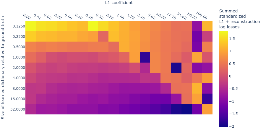
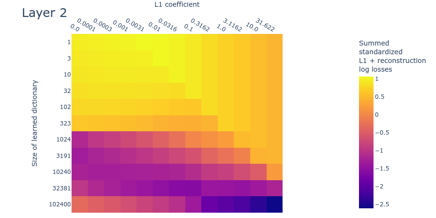
Below we plot the log reconstruction loss and log L1 penalty loss for different L1 penalty coefficients and dictionary sizes. The log losses are standardized by subtracting their means and dividing by their standard deviations (ignoring undefined values where we’d be taking the logarithm of $0$ L1 regularization loss) to put them on similar scales. As we saw in the MMCS plots (figure 3), there is an interaction between the L1 penalty coefficient and the reconstruction loss, as we see in these standardized log loss heatmaps for reconstruction loss (figure 7) and L1 regularization loss (figure 8) respectively:

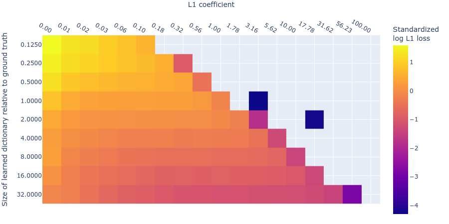
We can combine these two log loss plots by simply adding them together (which we can do because they are both standardized) to create the summed standardized L1 and reconstruction log loss (SSLL). In the SSLL plot (figure 9) we can see the same diagonal line as in figure 3 that indicates when the L1 parameter is too high. Using this plot to determine the right dictionary size is harder. Notice that there are curves of equivalent SSLL bending up from the bottom left (low L1 penalty coefficient, large dictionary size). We might be able to use the peaks of the curves to identify hyperparameters where the ground truth features are recovered. The peaks correspond to the regions of ‘sticky’ loss, where the L1 penalty coefficient is optimal for that dictionary size. If the dictionary is too small, however, there is no peak because there is no optimal L1 penalty coefficient (because all sparsity damages reconstruction loss).  Loss stickiness thus presents another potential way to find an optimal L1 penalty coefficient and dictionary size. 

Method 3: Mean max cosine similarity between a dictionary and those larger than it

This method relies on the fact that there are many ways for a learned dictionary to be wrong, but only one way to be right. 

Suppose there are $G$ ground truth features. Let’s consider what the mean max cosine similarity will be between two differently initialized dictionaries in multiple different cases. In cases where the dictionaries are different sizes, assume we’re always comparing all features in the smaller dictionary with the most similar feature in the larger dictionary.

1. Both dictionaries are the right size: Two separately initialized dictionaries with $G$ learnable features will learn the ground truth features and thus, after training, have the maximum possible mean max cosine similarity with each other. 
2. One dictionary is too small: Suppose one dictionary were too small, having instead only (say) $G/2$ learnable features. The mean max cosine similarity between these dictionaries will be lower than if both dictionaries are the right size, since the smaller dictionary won’t have learned the ground truth features and will instead have learned combinations of (likely correlated) features (or only the most common ground truth features). 
3. One dictionary is too large: Now suppose one of the dictionaries were instead too large, having (say) $2G$ learnable features. Now both dictionaries will learn the ground truth features, and the too-large autoencoder will have several ‘dead’ neurons (due to the L1 penalty) and/or repetitions of the same feature (though all but one of these will probably be ‘killed’ in favour of the most accurate replicate). Since a feature activated by the dead neurons is unlikely to have exactly recovered a ground truth feature before their neuron died, they will not be as similar to the ground truth features as the alive neurons. They will therefore be ignored by the mean max cosine similarity measure, since it takes only the maximum for each of the features in the smaller dictionary. Mean max cosine similarity should therefore be approximately the same as in case 1 (the theoretical maximum). 
4. Both dictionaries are too large: In the scenarios discussed above, a dictionary with $2G$ learnable features will learn the ground truth features (assuming it has the right L1 penalty coefficient) and have a bunch of dead neurons. The same is true for a dictionary with $4G$ features, which will have even more dead neurons. The features of the dead neurons will not be as similar to each other as features that match the ground truth. Therefore the mean max cosine similarity between a dictionary of $2G$ features and one with $4G$ features will be high, but not as high as between dictionaries of size $G$ and $nG$ (where $n$ is any positive integer). 

The above four cases describe in theory how we can identify dictionaries of the right size: When we compare each trained dictionary with all those dictionaries that are larger than it, the mean max cosine similarity should peak where the smaller dictionary is the right size and where L1 is at its optimum value. We find this empirically to be the case, indicating that we can perhaps use this quantity to search for good hyperparameters. 

Identifying the overcomplete feature basis used in a language model

We proposed three different methods that might let us identify the optimal dictionary size and L1 penalty coefficient for sparse autoencoders without access to the ground truth features that we want to recover. Armed with these methods, we now apply sparse autoencoders to real neural data from a small 6 layer transformer. 

Here we’ll look at the dead neurons, loss stickiness, and MMCS between each dictionary and those larger than it, measured on real data for dictionaries with different L1 penalty coefficients and dictionary sizes. If the toy data are a good model for the real data, then the plots should look similar in both cases. Unfortunately, at this interim stage in the project, the plots are sufficiently different that we can’t be sure whether we’ve got the right hyperparameters for recovering the inaccessible ‘ground truth’ features in the real data. Here we compare the plots for the toy data to the plots obtained by training our sparse autoencoder on the neural activations in the MLP. We show the result for layer 1 (i.e. the 2nd layer) of the language model since it’s roughly representative of the other layers. We include the plots for the other layers in the appendix.

Dead neurons

The dead neuron plot (figure 11) differs from the corresponding toy model plot (figure 4) primarily in that dead neurons are not observed even in the largest dictionaries. This could be because we haven’t used large enough dictionaries. If this is the case (and we’re not yet sure if it is), it means that the $256$-dimensional residual stream is capable of representing over $102400$ features in superposition. This implies a scaling factor of over $400$ features in superposition per residual dimension, which would be… a lot of superposition. Technically this would be possible due to the very high (exponential) limit suggested by the Johnson-Lindenstraus lemma. It might not even be that surprising if networks were using this many features; the input vocabulary size is already on the same order ($50304$).
 

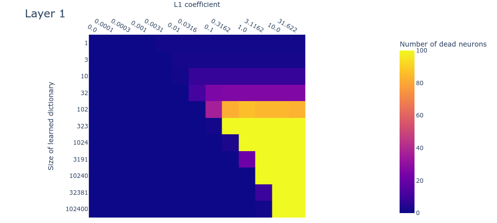
This is only an interim research result, so take this plot with a very heavy pinch of salt. We’re exploring various hypotheses, including the hypothesis that we have in fact used large enough dictionaries, but that we’re not seeing dead neurons for some other reason, such as irreducible noise in the data or something else. 

Loss stickiness

The SSLL plot (figure 12) looks somewhat different to the toy data plot (figure 9). That said, it still exhibits the diagonal line that indicates where the L1 penalty coefficient is too high. As we increase dictionary size, there is a sharp drop in the loss at around $1024$ features. There appears to be a flat region of SSLL surrounded by higher SSLL for the dictionaries of size $32381$ over a wide range of L1 penalty coefficients. But there are no obvious peaks of loss. It may be that we're simply using dictionaries that are too small. Overall, the plot is too different from the corresponding toy data plot to draw confident estimates for dictionary size. 

Mean max cosine similarity between a dictionary and those larger than it

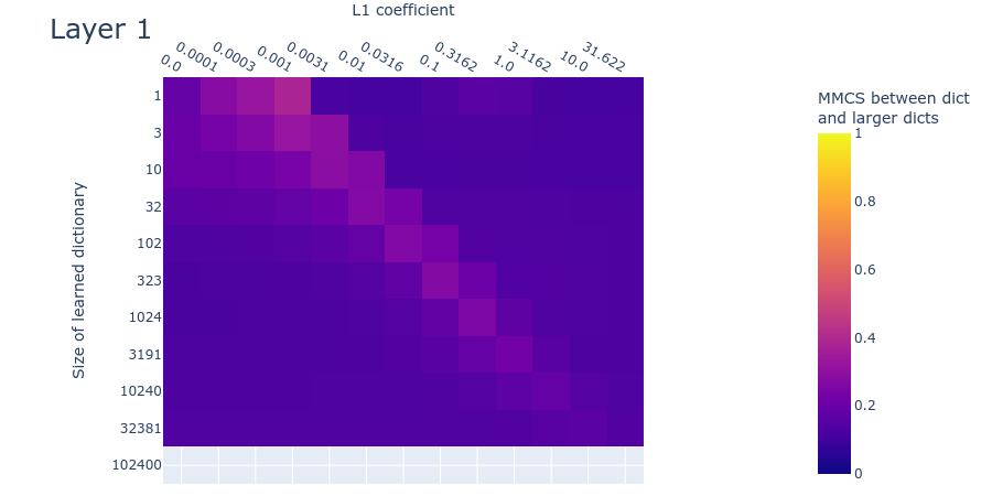
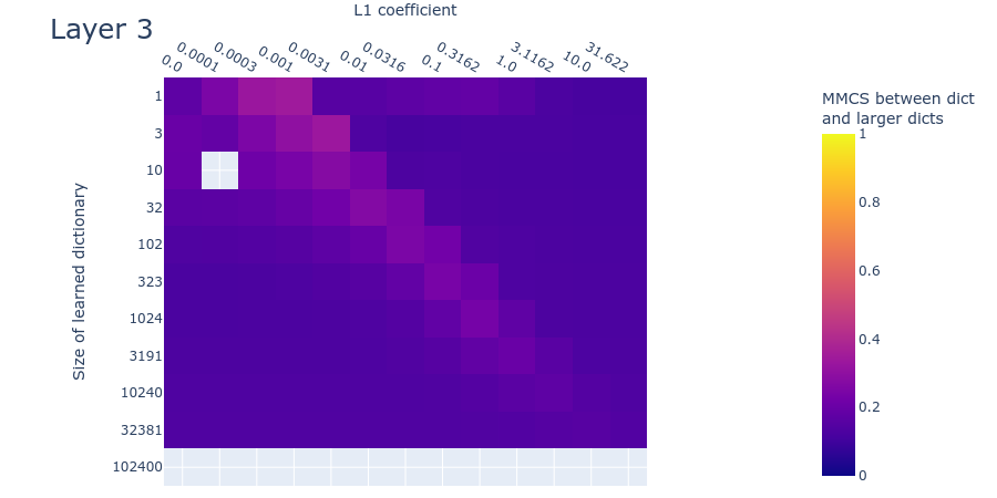
The MMCS plot (figure 13) is quite different from the toy data plot (figure 10). The MMCS between dictionaries never exceeds ~$0.4$. This means that the features learned in dictionaries of different sizes are often quite different. This is another indication that we’re possibly dealing with a much noisier dataset than the toy data. If so, the differences compared with the toy data plots might be remediable by training multiple dictionaries with different initializations and/or different activation datasets and then taking the average of the most similar features. An alternative possible remedy is to train the dictionaries for longer, if their features haven’t converged (even though their loss approximately has). Despite the faintness, both the toy data and this plot for real data nevertheless exhibit a ‘finger’ of elevated MMCS. But it’s unclear if we’ve seen the end of the finger; it may well continue beyond $102400$ features. As with the SSLL plot (Figure 12), it’s difficult to draw firm conclusions about the optimal dictionary size from the MMCS plot. 

Conclusion

We want to emphasize again that this is only an interim research report. We decided to post this primarily to spread the knowledge that no fancy sparse coding methods are needed to recover ground truth features (at least in toy data), as well as to elicit early feedback on our work. Code will be included in any final research report we decide to publish; we didn’t include it here to reduce the overhead of publishing interim research results.

We’ll probably continue this line of research. One of the main things we’d like to identify are the properties of the language model activations that cause the differences from the toy model in the plots of dead neurons, summed standardized log losses, and MMCS for different L1 penalty coefficients and dictionary sizes. Some potential reasons are:

• Simply not using large enough autoencoders – i.e. the expansion factor in the langauge model is larger than any we tested. 
• Experimental error, such as failing to train the autoencoder features to convergence, even though their losses were approximately converged.
• The lack of consistent ‘ground truth’ features in real language model data. A feature might be better represented by a distribution over directions, rather than by a single direction. It might be possible to model this in our toy data experiments by adding jitter to the ground truth feature directions during generation of the toy dataset.
• Real data may have irreducible background noise that makes it harder to learn the ground truth features. We might be able to model this in the toy data by adding noise vectors to both the labels and the inputs to the autoencoders (This is simply a different type of noise than adding jitter during feature construction). 
• The ground truth features were sampled uniformly from a hypersphere, which admits features that have dimensions with negative values. MLP activations (which we studied here) are usually positive. We could instead sample ground truth features from a strictly positive distribution. Or we could study the residual stream activations instead, which may be positive or negative. 
• We used a very limited amount of superposition in our toy data ($2\times$ as many features as dimensions). Adding more might capture more of the properties of the real data.
• We might have failed to capture the important statistical properties of the data: For instance, we didn’t explore different levels of feature correlations. Also, perhaps our feature probability decay was too low such that there wasn’t a large enough variation in feature probability.

If we continue this line of research, we’ll probably also explore better metrics for ground truth feature recovery than mean max cosine similarity. Currently, MMCS only accounts for the maximally similar dictionary element for each ground truth element. But dictionaries may have learned redundant copies of ground truth features, which MMCS fails to account for. An improved metric may be especially important if we explore variable levels of feature correlation and more variable differences between features’ probabilities (i.e. feature probability decay). MMCS also relies on cosine similarity, which will scale poorly as the sizes of our dictionaries increase for realistic models. 

It would be nice to know if the difference we’re seeing between the toy data and the langauge model results are due to there simply being too many features being in superposition in the langauge model or if it’s due to something about MLP activations in transformers. One way we could address this in future experiments is to train a transformer on a simpler, algorithmic task, rather than natural language. Algorithmic tasks can have fewer features than in natural language, so we might see less superposition as well as be able to precisely quantify probable ranges of feature sparsity.

At this point in the project, it’s worth reflecting on whether or not we should continue with it in light of our AI safety goals. We believe that we can make progress on the remaining problems on this topic. It will probably not be a major research effort to identify how language model data differs from the toy data, nor a major engineering effort to train dictionaries that are almost as large as practically possible. If we can do that, then it will probably be possible to identify the ground truth features used by small language models, insofar as they exist. This will be useful scientifically, since it would open up the possibility to study the structure of computation in language models. 

However, at least using this method of sparse coding, it’s extremely costly to extract features from superposition. Here, in our experiments on a small language model, we collected a lot of activations (our training runs required storing ~$15$M residual stream vectors of size $256$; ~$8$GB in bfloat16 for a single layer) and trained autoencoders that were many times larger than the MLPs we were studying. Here we found very weak, tentative evidence that, for a model of size $d_{model}=256$, the number of features in superposition was over $100,000$. This is a large scaling factor, and it’s only a lower bound. If the estimated scaling factor is approximately correct (and, we emphasize, we’re not at all confident in that result yet) or if it gets larger, then this method of feature extraction is going to be very costly to scale to the largest models – possibly more costly than training the models themselves. Continuing along this line of research might let us see just how costly it will be, and thus get a gauge of its feasibility. But we need to bear in mind that the research might ultimately not be useful for interpreting models that push the frontiers of capabilities, especially if we want to interpret the models frequently during training, which is pretty important! 

If post hoc sparse coding turns out not to be a viable strategy for resolving superposition in large models, how should we proceed? The alternative, as Anthropic laid out in ‘The Strategic Picture of Superposition’ in their recent paper, is to build models without superposition. Building models without superposition (or models where features in superposition are easier to extract) looks increasingly attractive to us as the realities of using sparse coding to interpret a model become clearer. Even if we do pursue models without superposition, it’s still possible that this investigation of sparse coding is worth continuing: Models without superposition are likely to be very sparse, and therefore a project that helps us understand how neural networks structure their sparsely coded features may help us build models that don’t have superposition. 

 

Appendix

Denoising autoencoders (with the right amount of noise) are sparse autoencoders that recover ground truth features

A recent paper from Bricken et al. (2022) indicated that denoising autoencoders learn sparse features. Our experiments show that they, too, recover the ground truth features. We thought we might be able to use denoising autoencoders to make our search for the right L1 penalty coefficient easier: We thought that the range of acceptable L1 penalties might be wider when there is a small amount of noise, thus making the acceptable range easier to find. To our surprise, we found little interaction between the L1 penalty coefficient and noise standard deviation:

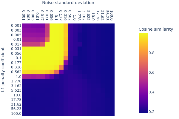
 The appropriate range for the noise standard deviation (with respect to the mean max cosine similarity) was also narrower than L1 penalty coefficient. We decided not to use noise in our experiments in order to avoid having to search through another (more sensitive) hyperparameter. Moreover, the denoising autoencoders usually had a very slightly worse mean max cosine similarity than their noiseless L1 counterparts. 

Note that for this particular experiment, all ground truth features had the same probability of being included in a datapoint and there were no correlations between features. The dictionary size was fixed at $512$, which is the same as the number of ground truth features. 

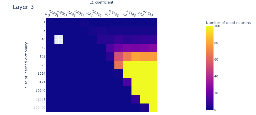
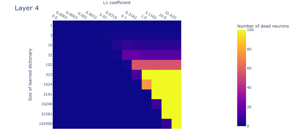
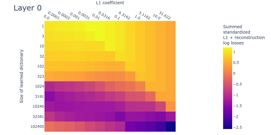
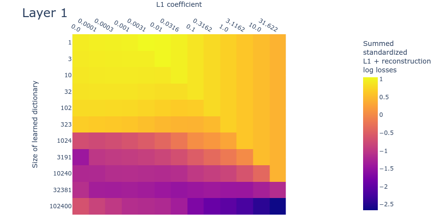
Heatmaps for L1 penalty coefficient vs Dictionary size for all layers

Dead neurons

 

Loss stickiness

Mean max cosine similarity between a dictionary and those larger than it

23 comments

Comments sorted by top scores.