UML XII: Dimensionality Reduction

post by Rafael Harth (sil-ver) · 2020-02-23T19:44:23.956Z · LW · GW · 0 comments

Contents

  I
  II
  III
  IV
  V
  VI
  VII
  VIII
  IX
  X
None
No comments

(This is the twelfth post in a sequence on Machine Learning based on this book. Click here [? · GW] for part I.)

This post will be more on the mathy side (all of it linear algebra). It contains orthonormal matrices, eigenvalues and eigenvectors, and singular value decomposition.

I

Almost everything I've written about in this series thus far has been about what is called supervised learning, which just means "learning based on a fixed amount of training data." This even includes most of the theoretical work from chapters I-III, such as the PAC learning model. On the other side, there is also unsupervised learning, which is learning without any training data.

Dimensionality reduction is about taking data that is represented by vectors in some high-dimensional space and converting them to vectors in a lower-dimensional space, in a way that preserves meaningful properties of the data. One use case is to overcome computational hurdles in supervised learning – many algorithms have runtimes that increase exponentially with the dimension. In that case, we would essentially be doing the opposite of what we've covered in the second half of post VIII [LW · GW], which was about increasing the dimensionality of a data set to make it more expressive. However, dimensionality reduction can also be applied to unsupervised learning – or even to tasks that are outside of machine learning altogether. I once took a class on Information Visualization, and they covered the technique we're going to look at in this post (although "covered" did not include anyone understanding what happens on a mathematical level). It is very difficult to visualize high-dimensional data; a reasonable approach to deal with this problem is to map it into 2d space, or perhaps 3d space, and then see whether there are any interesting patterns.

The aforementioned technique is called principal component analysis. I like it for two reasons: one, linear algebra plays a crucial role in actually finding the solution (rather than just proving some convergence bound); and two, even though the formalization of our problem will look quite natural, the solution turns out to have highly elegant structure. It's an example of advanced concepts naturally falling out of studying a practical problem.

II

Here is the outline of how we'll proceed:

• Define the setting
• Specify a formal optimization problem that captures the objective "project the data into a lower-dimensional space while losing as little information as possible"
• Prove that the solution has important structure
• Prove that it has even more important structure
• Repeat steps #3 and #4

At that point, finding an algorithm that solves the problem will be trivial.

III

Let $n,d\in N_{+}$ with $d>n$ and let $(x_1,...,x_m)$ be some data set, where $x_i\in R^d$ for all $i\in \left[m\right]$. We don't assume the data has labels this time since we'll have no use for them. (As mentioned, dimensionality reduction isn't restricted to supervised learning.)

We now wish to find a linear map $\varphi :R^d\to R^n$ that will project our data points into the smaller space $R^n$ while somehow not losing much information and another linear map $\psi :R^n\to R^d$ that will approximately recover it.

The requirement that $\varphi$ be linear is a pretty natural one. The sets $R^d$ and $R^n$ are bijective, so if arbitrary functions are allowed, it is possible to define $\varphi$ in such a way that no information is lost. However, if you've ever seen a bijection between $R$ and $R^2$ written out, you'll know that this is a complete non-starter (such functions do not preserve any intuitive notion of structure).

Another way to motivate the requirement is by noting how much is gained by prescribing linearity. The space of all functions between two sets is unfathomably vast, and linearity is a strong and well-understood property. If we assume a linear map, we can make much faster progress.

IV

Since we are assuming linearity, we can represent our linear maps as matrices. Thus, we are looking for a pair $(A,B)$, where $A$ is an $n\times d$ matrix and $B$ a $d\times n$ matrix.

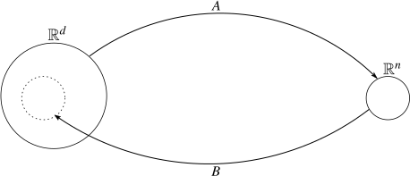
The requirement that the mapping loses as little information as possible can be measured by how well we can recover the original data. Thus, we assume our data points are first mapped to $R^n$ according to $A$, then mapped back to $R^d$ according to $B$, and we measure how much the points have changed. (Of course, also we square every distance because mathematicians love to square distances.) This leads to the objective

$\text{arg}{min}_{A\in {\text{Mat}}_{n,d},B\in {\text{Mat}}_{d,n}}{\sum }_{i=1}^m||x_i-BA{x}_i|{|}^2$ .

We say that the pair $(A,B)$ is a solution to our problem iff it is in the argmin above.

V

Before we go about establishing the first structural property of our solution, let's talk about matrices and matrix multiplication.

---

There are (at least) two different views one can take on matrices and matrix multiplication. The common one is what I hereby call the computational view because it emphasizes how matrix-vector and matrix-matrix multiplication is realized – namely, like this:

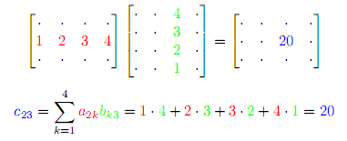
In this view, matrices and linear maps are sort of the same thing, at least in the sense that both can be applied to vectors.

Since reading Linear Algebra Done Right [LW · GW], I've become increasingly convinced that emphasizing the computational view is a bad idea. The alternative perspective is what I hereby call the formal view because it is closer to the formal definition. Under this view, a matrix is a rectangular grid of numbers:

$\left[\begin{array}{ccc}{a}_{1,1}& \cdots & a_{1,m}\\ ⋮& & ⋮\\ a_{n,1}& \cdots & a_{n,m}\end{array}\right]$

This grid (along with the bases of the domain space and target space) contains all the information about how a function works, but it is not itself a function. The crucial part here is that the first column of the matrix tells us how to write the first basis vector of the domain space as a linear combination of the target space, i.e., $\varphi \left(b_1\right)={\sum }_{i=1}^n{a}_{i,1}{b}_i^{\prime }$ if the two bases are $(b_1,...,b_m)$ and $(b_1^{\prime },...,b_n^{\prime })$. As far as this post is concerned, we only have two spaces, $R^d$ and $R^n$, and they both have their respective standard basis. Thus, if we assume $n=2$ and $d=3$ for the sake of an example, then the $d\times n$ matrix

$\left[\begin{array}{cc}1& 4\\ 2& 2\\ 5& 7\end{array}\right]$

tells us that the vector $(1,0)$ is mapped onto $(1,2,5)$ and the vector $(0,1)$ onto $(4,2,7)$. And that is all; this defines the linear map which corresponds to the matrix.

Another consequence of this view is that I exclusively draw matrices that have rectangular brackets rather than round brackets. But I'm not devoted to the formal view – we won't exclusively use it; instead, we will use whichever one is more useful for any given problem. And I won't actually go through the trouble of cleanly differentiating matrices and maps; we'll usually pretend that matrices can send vectors to places themselves.

---

With that out of the way, the first thing we will prove about our solution is that it takes the form $(\bullet ,V)$, where $V$ is a pseudo-orthonormal matrix. ("It takes the form" means "there is a pair in the argmin of our minimization problem that has this form.") A square matrix is orthonormal if its columns (or equivalently, its rows) are orthonormal to each other (if read as vectors). I.e., they all have inner product 0 with each other and have norm 1. However, there is also a variant of this property that can apply to a non-square matrix, and there is no standard terminology for such a matrix, so I call it pseudo-orthonormal. In our case, the matrix $V$ will do this thing:

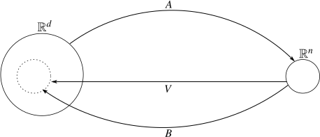
I.e., it will go from a small space to a larger space. Thus, it looks like this:

$\left[\begin{array}{ccc}{v}_{1,1}& \cdots & v_{1,n}\\ v_{2,1}& \cdots & v_{2,n}\\ ⋮& & ⋮\\ v_{d,1}& \cdots & v_{d,n}\end{array}\right]$

Or alternatively, this:

$\left[\begin{array}{ccc}{v}_1& \cdots & v_n\end{array}\right]$

where we write the entries as column vectors, i.e., $v_i=(v_{1,i}\cdots v_{d,i}{)}^T$.

For a proper orthonormal matrix, both the column vectors and the row vectors are orthonormal. For a $d\times n$ pseudo-orthonormal matrix, just the $v_i$ (i.e., the column vectors) are orthonormal. The row vectors can't be (unless many of them are zero vectors) because they're linearly dependent; there are $d$ many, and they live in $n$-dimensional space.

For a square matrix, the requirement that it be orthogonal is equivalent to the equations $V^{T}V=I$ and $V{V}^T=I$, or simply $V^T=V^{-1}$. A $d\times n$ pseudo-orthonormal matrix isn't square and doesn't have an inverse, but the first of the two equations still holds (and is equivalent to the requirement that the matrix be pseudo-orthonormal). To see why, consider the matrix product in the computational view. Instead of flipping the first matrix, you can just imagine both side by side; but go vertical in both directions, i.e.:

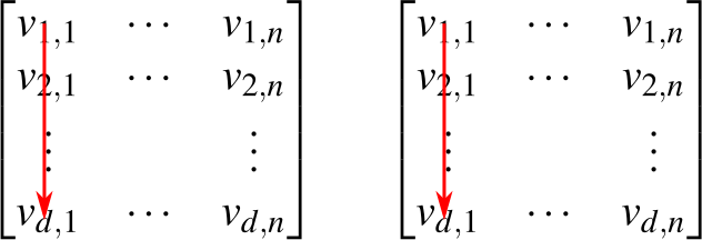
This shows that $(V^{T}V{)}_{k,\ell }=⟨v_k,v_{\ell }⟩$, and this is $1$ iff $k=\ell$ and 0 otherwise because the $v_i$ are orthonormal. Thus, $V^{T}V=I_n$.

Now recall that we wish to construct a pseudo-orthonormal matrix $V$ and prove that there exists a solution with $V$, i.e., a solution of the form $(\bullet ,V)$.

To construct $V$ note that $(1,0,...,0)$ is mapped to the first column vector of any matrix (formal view), and analogously for every other basis vector. It follows that the image of a matrix is just the span of the column vectors. Thus, $\text{im}\left(B\right)$ is an $n$-dimensional subspace of $R^d$, and we can choose an orthonormal basis $(v_1,...,v_n)$ of that subspace. Then we define $V:=\left[\begin{array}{ccc}{v}_1& \cdots & v_n\end{array}\right]$ as in the example above (only now the $v_i$ are the specific vectors from this orthonormal basis). Note that $V$ is indeed a $d\times n$ matrix. Clearly, both $V$ and $B$ have the same image (formal view).

We will also have use for $V^T$ (quite a lot, in fact). Let's add it into the picture:

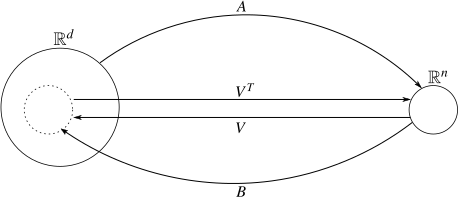
(Note that, even though the arrow for $V^T$ starts from the small circle, it can take vectors from all of $R^d$.)

We've established that $V^{T}V$ is the identity matrix, but $V{V}^T$ isn't. This can also be seen from this picture: $V{V}^T$ is a map from $R^d$ to $R^d$, but it maps all vectors into a subspace of $R^d$. Therefore, all vectors outside of the subspace have to be changed. But what about the vectors who are in the subspace? Could it be that it leaves those unchanged? The answer is affirmative; here's the proof:

Let $y\in \text{im}\left(V\right)$. Then $\exists z\in R^n$ such that $Vz=y$, and therefore, $V{V}^{T}y=V{V}^T\left(Vz\right)=V\left(V^{T}V\right)z=Vz=y$.

This fact is going to be important in just a second. Recall that we were here:

and we wanted to prove that there's a solution of the form $(\bullet ,V)$. Here's the proof:

Let $(A,B)$ be a solution. Then $BA$ is our optimal back-and-forth mapping. However, $BA=V{V}^{T}BA$, and, therefore, the pair $(AB{V}^T,V)$ is also an optimal back-and-forth mapping and thus is a solution.

Note that $BA=V{V}^{T}BA$ holds only because the matrix $BA$ sends all vectors into the subspace $\text{im}\left(B\right)$ which is the same as $\text{im}\left(V\right)$, and therefore $V{V}^T$ doesn't do anything.

VI

Next, we prove that there is a solution of the form $(V^T,V)$. We will do this by constructing a term that describes the distance we're trying to minimize and comparing its gradient to zero. Thus, we assume $x\in R^d$ and $y\in R^n$ and want to figure out how to choose $y$ such that the term $||x-Vy||$ is minimal. Using that $||a-b|{|}^2=⟨a,a⟩-2⟨a,b⟩+⟨b,b⟩$ and that $⟨a,b⟩=a^{T}b=b^{T}a$, we have:

$||x-Vy|{|}^2=x^{T}x-2y^T{V}^{T}x+y^T{V}^{T}Vy=||x|{|}^2-2y^T{V}^{T}x+||y|{|}^2$

The gradient of this term with respect to $y$ is $-2V^{T}x+2y$. Setting it to 0 yields $y=V^{T}x$. Thus, for each point $x\in R^d$, the vector $y$ in $R^n$ that will make the distance $||x-Vy||$ smallest has the form $V^{T}x$. In particular, this is true for all of our training points $x_i$. Since we have shown that there exists a solution of the form $(\bullet ,V)$, this implies that $(V^T,V)$ is such a solution.

VII

Before we prove that our solution has even more structure, let's reflect on what it means that it has the form $(V^T,V)$ with $V$ orthonormal. Most importantly, it means that the vectors we obtain are all orthogonal to each other (formal view). We call those vectors the principal components of our data set, which give the technique its name. You can think of them as indicating the directions that are most meaningful to capture what is going on in our data set. The more principal components we look at (i.e., the larger of an $n$ we choose), the more information we will preserve. Nonetheless, if a few directions already capture most of the variance in the data, then $(V^T,V)$ might be meaningful even though $n$ is small.

For more on this perspective, I recommend this video (on at least 1.5 speed).

VIII

Based on what we have established, we can write our optimization problem as

$\text{arg}{min}_{V\in {\text{Mat}}_{d,n},V\text{orthonormal}}{\sum }_{i=1}^m||x_i-V{V}^T{x}_i|{|}^2$

Looking at just one of our $x_i$, we can rewrite the distance term like so:

$||x_i-V{V}^T{x}_i||=||x_i|{|}^2-2{x_i}^{T}V{V}^T{x}_i+{x_i}^{T}V{V}^{T}V{V}^T{x}_i=||x_i|{|}^2-{x_i}^{T}V{V}^T{x}_i$

then, since $||x_i|{|}^2$ does not depend on $V$, we can further rewrite our problem as

$\text{arg}{max}_{V\in {\text{Mat}}_{d,n},V\text{orthonormal}}{\sum }_{i=1}^m{x_i}^{T}V{V}^T{x}_i$

Now we perform a magic trick. The term ${x_i}^{T}V{V}^T{x}_i$ may just be considered a number, but it can also be considered a $1\times 1$ matrix. In that case, it is equal to its trace. (The trace of a square matrix is the sum of its diagonal entries). The trace has the property that one can "rotate" the matrix product it is applied to, so

$\text{trace}(M_1,...,M_n)=\text{trace}(M_2,...,M_n,M_1)$

(This follows from the fact that $\text{trace}\left(AB\right)=\text{trace}\left(BA\right)$, which is easy to prove.) It also has the property that, if $A^{T}B$ is square (but $A$ and $B$ are not), $\text{trace}\left(A^{T}B\right)=\text{trace}\left(A{B}^T\right)$; this will be important later. If we apply rotation to our case, we get

${x_i}^{T}V{V}^T{x}_i=\text{trace}\left({x_i}^{T}V{V}^T{x}_i\right)=\text{trace}\left(V{V}^T{x}_i{x_i}^T\right)=\text{trace}\left(V^T{x}_i{x_i}^{T}V\right)$

and, since the trace is linear,

${\sum }_{i=1}^m\text{trace}\left(V^T{x}_i{x_i}^{T}V\right)=\text{trace}(V^T({\sum }_{i=1}^m{x}_i{x_i}^T)V)$

The key component here is the matrix $X:=({\sum }_{i=1}^m{x}_i{x_i}^T)$. Note that $X$ does not depend on $V$. However, we will finish deriving our technique by showing that the columns of $V$ are precisely the $n$ eigenvectors of $X$ corresponding to its $n$ largest eigenvalues.

IX

Many matrices have something called a singular-value decomposition – this is a decomposition $X=SD{S}^{-1}$ such that $S$ consists of the eigenvectors of $X$ (column vectors) and $D$ is diagonal, i.e.:

$S=\left[\begin{array}{ccc}{w}_1& \cdots & w_d\end{array}\right]D=\left[\begin{array}{ccc}{\lambda }_1& & \\ & \ddots & \\ & & {\lambda }_d\end{array}\right]$

The matrix $D$ can be considered to represent the same function as $X$ but with regard to a different basis, namely the basis of the eigenvectors of $X$. Thus, the singular value decomposition exists iff there exists a basis that only consists of eigenvectors of $X$.

It is possible to check that the matrix $S$ which realizes this decomposition is, in fact, the matrix with the eigenvectors of $X$ as column vectors. Consider the first eigenpair $(w_1,{\lambda }_1)$ of $X$. We have $X{w}_1={\lambda }_1{w}_1$. On the other hand, $S$ sends the vector $(1,0,...,0)$ to $w_1$ (formal view), and therefore, $S^{-1}$ sends $w_1$ to $(1,0,...,0)$. Then $D$ sends $(1,0,...,0)$ to $(\lambda ,0,...,0)$ because it's a diagonal matrix, and $S$ sends $(\lambda ,0,...,0)$ to $\lambda S(1,0,...,0)$ which is $\lambda w_1$ (formal view). In summary,

$SD{S}^{-1}{w}_1=SD(1,0,...,0)=S(\lambda ,0,...,0)=\lambda w_1=X{w}_1$

This shows that $SD{S}^{-1}$ does the right things on the vectors $w_1,...,w_d$, which is already a proper proof that the decomposition works since $(w_1,...,w_d)$ is, by assumption, a basis of $R^d$.

In our case, $X$ is symmetric; this implies that there exists a decomposition such that $S$ is orthonormal. (We won't show this.) Note that, unlike $V$, the matrix $S$ is a square $d\times d$ matrix, hence $S^T=S^{-1}$ and the decomposition can be written as $X=SD{S}^T$.

Recall that the term we want to maximize is $\text{trace}\left(V^{T}XV\right)$. We can rewrite this as $V^{T}XV=V^{T}SD{S}^{T}V=\left[S^{T}V{]}^{T}D\right[S^{T}V]$. The matrix $\left[S^{T}V\right]$ is a $d\times n$ matrix, so not square, but it is pseudo-orthonormal since $\left[S^{T}V{]}^T\right[S^{T}V]=V^{T}S{S}^{T}V=V^{T}V=I$. Using the previously mentioned additional rules of the trace (which allow us to take the transpose of both $[S^{T}V{]}^{T}D$ and $\left[S^T\right]V$), we can write

$\text{trace}\left(V^{T}XV\right)=\text{trace}\left(\right[S^{T}V{]}^{T}D\left[S^{T}V\right])=\text{trace}(D\left[S^{T}V\right]\left[S^{T}V{]}^T\right)$

Multiplying any matrix with a diagonal $D$ from the left multiplies every entry in row $i$ with $D_{i,i}$, and in particular, multiplies the diagonal element $\left(\right[S^{T}V\left]\right[S^{T}V{]}^T{)}_{i,i}$ with $D_{i,i}$. Therefore, the above equals ${\sum }_{i=1}^d{D}_{i,i}\left(\right[S^{T}V\left]\right[S^{T}V{]}^T{)}_{i,i}$. Now recall that $\left[S^{T}V\right]$ is pseudo-orthonormal and looks like this:

$\left[\begin{array}{ccc}{z}_{1,1}& \cdots & z_{1,n}\\ z_{2,1}& \cdots & z_{2,n}\\ ⋮& & ⋮\\ z_{d_1}& \cdots & z_{d,n}\end{array}\right]$

The column vectors are properly orthonormal; they all have norm 1. The row vectors are not orthonormal, but if the matrix were extended to a proper $d\times d$ matrix, they would become orthonormal vectors. Thus, their norm is at most 1. However, the sum of all squared norms of row vectors equals the sum of all squared norms of column vectors (both are just the sum of every matrix entry squared), which is just $n$. It follows that each $\left(\right[S^{T}V\left]\right[S^{T}V{]}^T{)}_{i,i}$ is at most $1$, and the sum, namely ${\sum }_{i=1}^d\left(\right[S^{T}V\left]\right[S^{T}V{]}^T{)}_{i,i}$, is at most $n$. Now consider the term whose maximum we wish to compute:

${\sum }_{i=1}^d{D}_{i,i}\left(\right[S^{T}V\left]\right[S^{T}V{]}^T{)}_{i,i}$

Given the above constraints, the way to make it largest is to weigh the $n$ largest $D_{i,i}$with 1, and the rest with 0. It's not obvious that this can be achieved, but it is clear that it cannot get larger. Thus, ${\sum }_{i=1}^d{D}_{i,i}\left(\right[S^{T}V\left]\right[S^{T}V{]}^T{)}_{i,i}\le {\sum }_{i=1}^m{D}_{i,i}^{\ast }={\sum }_{i=1}^m{\lambda }_i^{\ast }$, where $D^{\ast }$ is $D$ reordered such that the largest $n$ eigenvalues, which we call ${\lambda }_1^{\ast },...,{\lambda }_n^{\ast }$, come first.

Now recall that we have previously written our term as $\text{trace}(V^T({\sum }_{i=1}^m{x}_i{x_i}^T)V)$ or equivalently $\text{trace}\left(V^{T}XV\right)$. If we choose $V=\left[\begin{array}{c}{w}_1^{\ast }\cdots w_n^{\ast }\end{array}\right]$ where $w_1^{\ast },...,w_n^{\ast }$ are the eigenvectors of $X$ corresponding to ${\lambda }_1^{\ast },...,{\lambda }_n^{\ast }$, we get $XV=X[w_1^{\ast }\cdots w_n^{\ast }]=[{\lambda }_1^{\ast }{w}_1^{\ast }\cdots {\lambda }_n^{\ast }{w}_n^{\ast }]$ and $V^{T}XV=V^T[{\lambda }_1{w}_1^{\ast }\cdots {\lambda }_n{w}_n^{\ast }]$. The $i$-th entry on the diagonal of this matrix is ${w_i^{\ast }}^T{\lambda }_i^{\ast }{w}_i^{\ast }={\lambda }_i^{\ast }||w_i^{\ast }|{|}^2={\lambda }_i^{\ast }$. Since we have established that this is an upper-bound, that makes this choice for $V$ a solution to our original problem, namely $\text{arg}{min}_{V\in {\text{Mat}}_{d,n},V\text{orthonormal}}{\sum }_{i=1}^m||x_i-V{V}^T{x}_i|{|}^2$.

X

As promised, the algorithm is now trivial – it fits into three lines:

Given $x_1,...,x_m\in R^d$, compute the matrix $X:={\sum }_{i=1}^m{x}_i{x_i}^T$, then compute the eigenvalues ${\lambda }_1,...,{\lambda }_d$ of $X$, with eigenvectors $w_1,...,w_d$. Take the $n$ eigenvectors with the largest eigenvalues and put them into a matrix $V$. Output $(V^T,V)$.

0 comments

Comments sorted by top scores.