Sparse autoencoders find composed features in small toy models
post by Evan Anders (evan-anders), Clement Neo (clement-neo), Jason Hoelscher-Obermaier (jas-ho), Jessica N. Howard (jnhoward) · 2024-03-14T18:00:43.339Z · LW · GW · 12 commentsContents
  Summary
  Introduction
  Experiment Details
    ReLU Output Toy Models
    Sparse Autoencoders (SAEs)
    Synthetic Data Vectors with Composed Features
      Including One-hot Vectors
  Results
    Correlated Feature Amplitudes
    Uncorrelated Feature Amplitudes
    Does a Cosine Similarity Loss Term Fix This Problem?
    What if the SAE Actually Gets to See the True Features?
  Takeaways
  Future work
  Code
  Acknowledgments
  Citing this post
None
12 comments
Summary
- Context: Sparse Autoencoders (SAEs) reveal interpretable features in the activation spaces of language models. They achieve sparse, interpretable features by minimizing a loss function which includes an penalty on the SAE hidden layer activations.
- Problem & Hypothesis: While the SAE penalty achieves sparsity, it has been argued [LW · GW] that it can also cause SAEs to learn commonly-composed features rather than the “true” features in the underlying data.
- Experiment: We propose a modified setup of Anthropic’s ReLU Output Toy Model where data vectors are made up of sets of composed features. We study the simplest possible version of this toy model with two hidden dimensions for ease of comparison to many of Anthropic’s visualizations.
- Features in a given set in our data are anticorrelated, and features are stored in antipodal pairs. Perhaps it’s a bit surprising that features are stored in superposition at all, because the features in the very small models we studied here are not sparse (they occur every-other data draw so have S ~ 0.5 in the language of Anthropic’s Toy Models paper)[1].
- Result: SAEs trained on the activations of these small toy models find composed features rather than the true features, regardless of learning rate or coefficient used in SAE training.
- This finding largely persists even when we allow the SAE to see one-hot vectors of true features 75% of the time.
- Future work: We see these models as a simple testing ground for proposed SAE training modifications. We share our code in the hopes that we can figure out, as a community, how to train SAEs that aren’t susceptible to this failure mode.
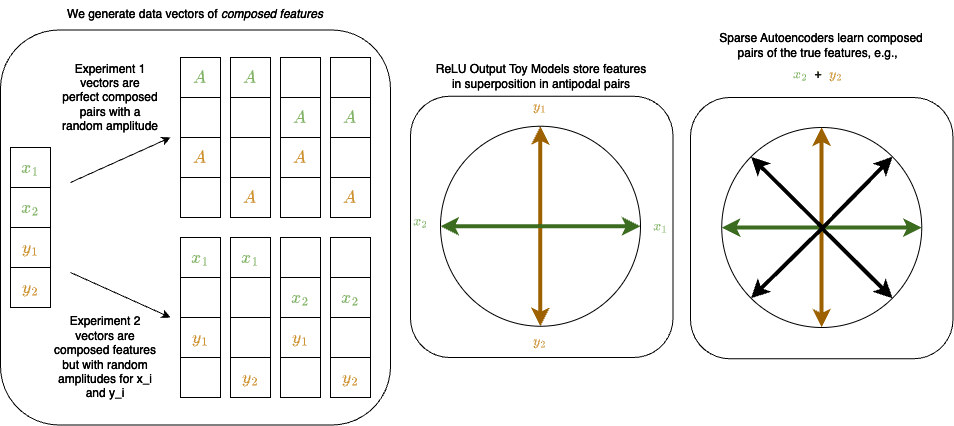
The diagram below gives a quick overview of what we studied and learned in this post:
Introduction
Last year, Anthropic and EleutherAI/Lee Sharkey's MATS stream showed that sparse autoencoders (SAEs) find human-interpretable “features” in language model activations. They achieve this interpretability by having sparse activations in the SAE hidden layer, such that only a small number of SAE features are active for any given token in the input data. While the objective of SAEs is, schematically, to “reconstruct model activations perfectly and do so while only having a few true features active on any given token,” the loss function used to train SAEs is a combination of mean squared error reconstruction of model activations and an penalty on the SAE hidden layer activations. This term may introduce unintended “bugs” or failure modes into the learned features.
Recently, Demian Till [LW · GW] questioned whether SAEs find “true” features. That post argued that the penalty could push autoencoders to learn common combinations of features, because having two common true features which occur together shoved into one SAE feature would achieve a lower value of the term in the loss than two independent “true” features which fire together.
This is a compelling argument, and if we want to use SAEs to find true features in natural language, we need to understand when this failure mode occurs and whether we can avoid it. Without any knowledge of what the true features are in language models, it’s hard to evaluate how robust of a pitfall this is for SAEs, and it’s also hard to test if proposed solutions to this problem actually work at recovering true features (rather than just a different set of not-quite-right ones). In this post, we turn to toy models, where the true features are known, to determine:
- Do SAEs actually learn composed features (common feature combinations)?
- If this happens, when does it happen and how can we fix it?
In this blog post, we’ll focus on question #1 in an extremely simple toy model (Anthropic’s ReLU output model with 2 hidden dimensions) to argue that, yes, SAEs definitely learn composed (rather than true) features in a simple, controlled setting. We release the code that we use to create the models and plots in the hope that we as a community can use these toy models to test out different approaches to fixing this problem, and we hope to write future blog posts that help answer question #2 above (see Future Work section).
The synthetic data that we use in our toy model is inspired by this post by Chris Olah about feature composition. In that post, two categories of features are considered: shapes and colors. The set of shapes is {circle, triangle, square} and the set of colors is {white, red, green, blue, black}. Each data vector is some (color, shape) pair like (green, circle) or (red, triangle). We imagine that these kinds of composed features occur frequently in natural datasets. For example, we know that vision models learn to detect both curves and frequency (among many other things), but you could imagine curved shapes with regular patterns (see: google search for ‘round gingham tablecloth’). We want to understand what models and SAEs do with this kind of data.
Experiment Details
ReLU Output Toy Models
We study Anthropic’s ReLU output model:
Here the model weights and bias are learned. The model inputs are generated according to a procedure we lay out below in the “Synthetic Data Vectors with Composed Features” section, and the goal of the model is to reconstruct the inputs. We train these toy models using the AdamW optimizer with learning rate , weight decay , , and . Training occurs over batches where each batch contains data vectors. The optimizer minimizes the mean squared error loss:
Sparse Autoencoders (SAEs)
We train sparse autoencoders to reconstruct the hidden layer activations of the toy models. The architecture of the SAEs is:
Where the encoding weights and bias and decoding weights W and bias are learned.
Sparse autoencoders (SAEs) are difficult to train. The goals of training SAEs are to:
- Create a model which captures the full variability of the baseline model that it is being used to interpret.
- Create a model which is sparse (that is, it has few active neurons and thus a low norm for any feature vector input, and its neurons are monosemantic and interpretable).
To achieve these ends, SAEs are trained on the mean squared error of reconstruction of model activations (a proxy for goal 1) and are trained to minimize the \ell_1 norm of SAE activations (a proxy for goal 2).
We follow advice from Anthropic’s January and February updates in informing our training procedure.
In this work, we train SAEs using the Adam optimizer with and and with learning rates . We minimize the mean of the fractional variance explained (FVE) and the norm of the SAE hidden layer feature activations, so our loss function is
The goal of minimizing the FVE instead of a standard squared error is to ensure our SAE is agnostic to the size of the hidden layer of the model it is reconstructing (so that a terrible reconstruction always scores 1 regardless of dimensionality)[2]. We vary the damping coefficient . The SAEs are trained over total data samples in batches sizes of for a total of batches. The learning rate linearly warms up from 0 over the first 10% of training and linearly cools down to 0 over the last 20% of training. At each training step, the columns of the decoder matrix are all normalized to 1; this keeps the model from "cheating'' on the penalty (otherwise the model would create large outputs using small activations with large decoder weights).
Synthetic Data Vectors with Composed Features
A primary goal of studying a toy model is to learn something universal about larger, more complex models in a controlled setting. It is therefore critical to reproduce the key properties of natural language that we are interested in studying in the synthetic data used to train our model.
The training data used in natural language has the following properties:
- There are many more features in the data than there are dimensions in the model.
- Most features in the dataset appear rarely (they are sparse).
- Some features appear more frequently than others (the probability of features occurring is a non-uniform distribution and the most-frequently-occurring and least-frequently-occurring features have wildly different probabilities).
- Features do not appear in isolation. We speculate that features often appear in composition in natural language datasets.
- For example, a subset of words in a sentence can have a specific semantic meaning while also being in a specific grammatical context (e.g., inside a set of parentheses or quotation marks).
- It’s possible that token in context features are an example of composed features. For example, it’s possible that the word “the” is a feature, and the context “mathematical text” is a feature, and “the word ‘the’ in the context of mathematical text” is a composition of these features.
In this post, we will focus on data vectors that satisfy #1 and #4 above and we hope to satisfy #2 and #3 in future work. To create synthetic data, we largely follow prior work [Jermyn+2022, Elhage+2022] and generate input vectors , where each dimension is a “feature'' in the data. We consider a general form of data vectors composed of m sub-vectors where those sub-vectors represent independent feature sets, and where each subvector has exactly one non-zero element so that ; dimensionally, with .
In this blog post, we study the simplest possible case: two sets () each of two features so that data vectors take the form . Since these features occur in composed pairs, in addition to there being four true underlying features there are also four possible feature configurations that the models can learn: and . For this case, a 2-dimensional probability table exists for each composed feature pair giving the probability of occurrence of each composed feature set where and . We consider uniformly distributed, uncorrelated features, so that the probability of any set of features being present is uniform and is , so the simple probability table for our small model is:
| 0.25 | 0.25 | |
| 0.25 | 0.25 |
The correlation between a feature pair can be raised by increasing while lowering the probability of appearing alongside and the probability of appearing alongside (and properly normalizing the rest of the probability table). This is interesting and we want to do this in future work, but in this specific post we’ll mostly just focus on the simple probability table above.
To generate synthetic data vectors , we randomly sample a composed pair from the probability table. We draw the magnitudes of these features from uniform distributions, and . We can optionally correlate the amplitudes of these features using a correlation coefficient by setting . Note that by definition, all features in are anticorrelated since they never co-occur, and the same is true of all features in . In this post, we study two cases:
- for perfectly correlated feature amplitudes.
- for perfectly uncorrelated feature amplitudes.
Including One-hot Vectors
In the experiments outlined above, all data vectors are two-hot, containing a nonzero value in some and a nonzero value in some . One could argue that, for that data, regardless of , the natural basis of the data is actually composed pairs and the underlying “true” features are less relevant.
We will therefore consider a case where there is some probability that a given data vector only contains one or one – but not both. We looked at , but in this blog post we will only display results from the case. To generate the probability table for these data, the table from above is scaled by , then an additional row and column are added showing that each feature is equally likely to be present in a one-hot vector (and those equal probabilities must sum up to ). An example probability table for is:
| 0.0625 | 0.0625 | 0.1875 | |
| 0.0625 | 0.0625 | 0.1875 | |
| 0.1875 | 0.1875 | 0 |
Results
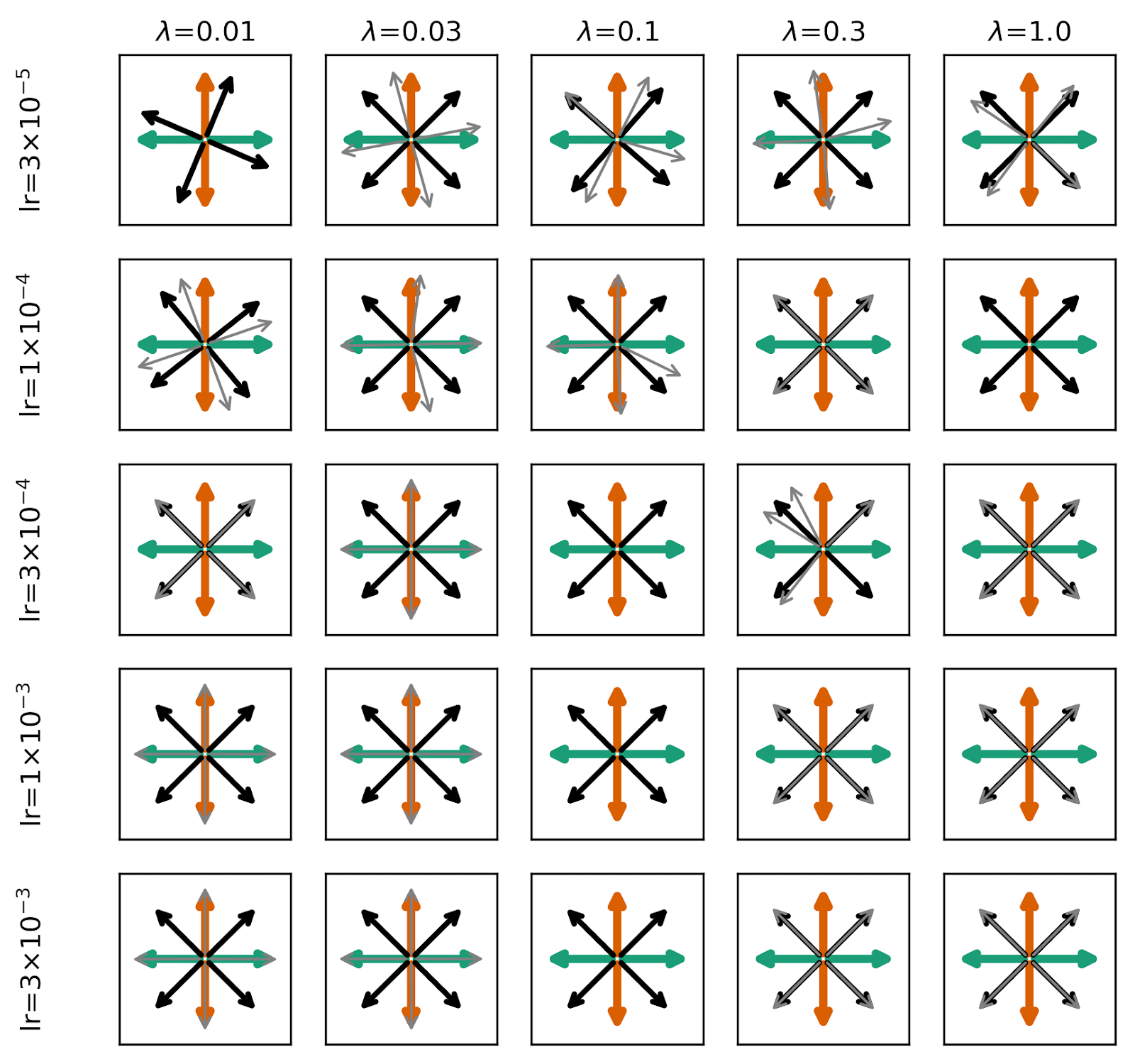
Correlated Feature Amplitudes
We begin with a case where the amplitudes of the features are perfectly correlated such that the four possible data vectors are , , , and with . Yes, this is contrived. The data vectors here are always perfect composed pairs. In some ways we should expect SAEs to find those composed pairs, because those are probably a more natural basis for the data than the "true" features we know about.
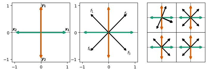
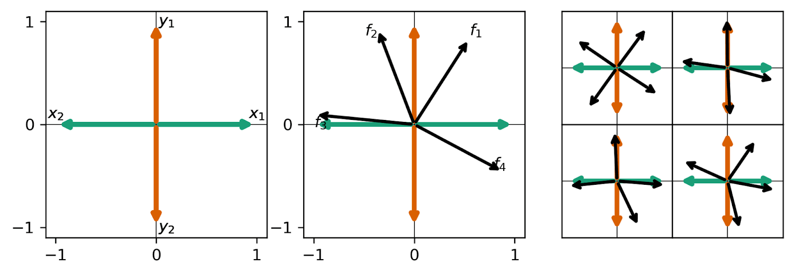
As mentioned above, we study the case where the ReLU output model has two hidden dimensions, so that we can visualize the learned features by visualizing the columns of the learned weight matrix in the same manner as Anthropic’s work (e.g., here). An example of a model after training is shown in the left panel of this figure:
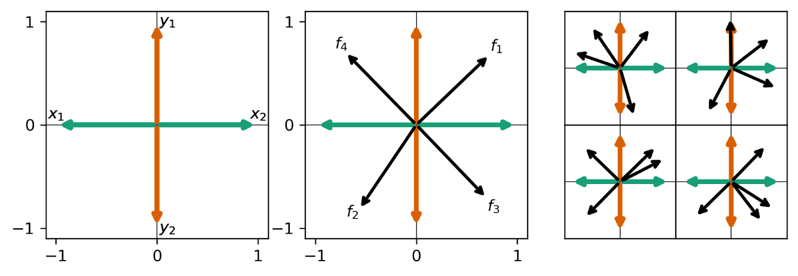
The features in the left panel are labeled by their and , and all features are rotated for visualization purposes so that the features are on the x-axis. We find the same antipodal feature storage as Anthropic observed for anticorrelated features -- and this makes sense! Recall that in our data setup, and are definitionally anticorrelated, and so too are and . Something that is surprising is that the model chooses to store these features in superposition at all! These data vectors are not sparse.[1] Each feature occurs in every other data vector on average. For a single set of uncorrelated features, models only store features in superposition when the features are sparse. Here, the model takes advantage of the nature of the composed sets and uses superposition despite a lack of sparsity.
We train five realizations of SAEs on the hidden layer activations of this toy model with a learning rate of and regularization coefficient . Of these SAEs, the one which achieves the lowest loss (reconstruction + ) is plotted in the large middle panel in the figure above (black arrows, overlaid on the model’s feature representations). This SAE’s features are labeled according to their hidden dimension in the SAE, so here e.g., is a composed feature of and like . The other four higher-loss realizations are plotted in the four rightmost sub-panels. We find a strong preference for off-axis features – which is to say, the SAE learns composed pairs. Each of the five realizations we study (middle and right panels) have this flaw, with only one realization finding even a single true underlying feature (upper right panel).
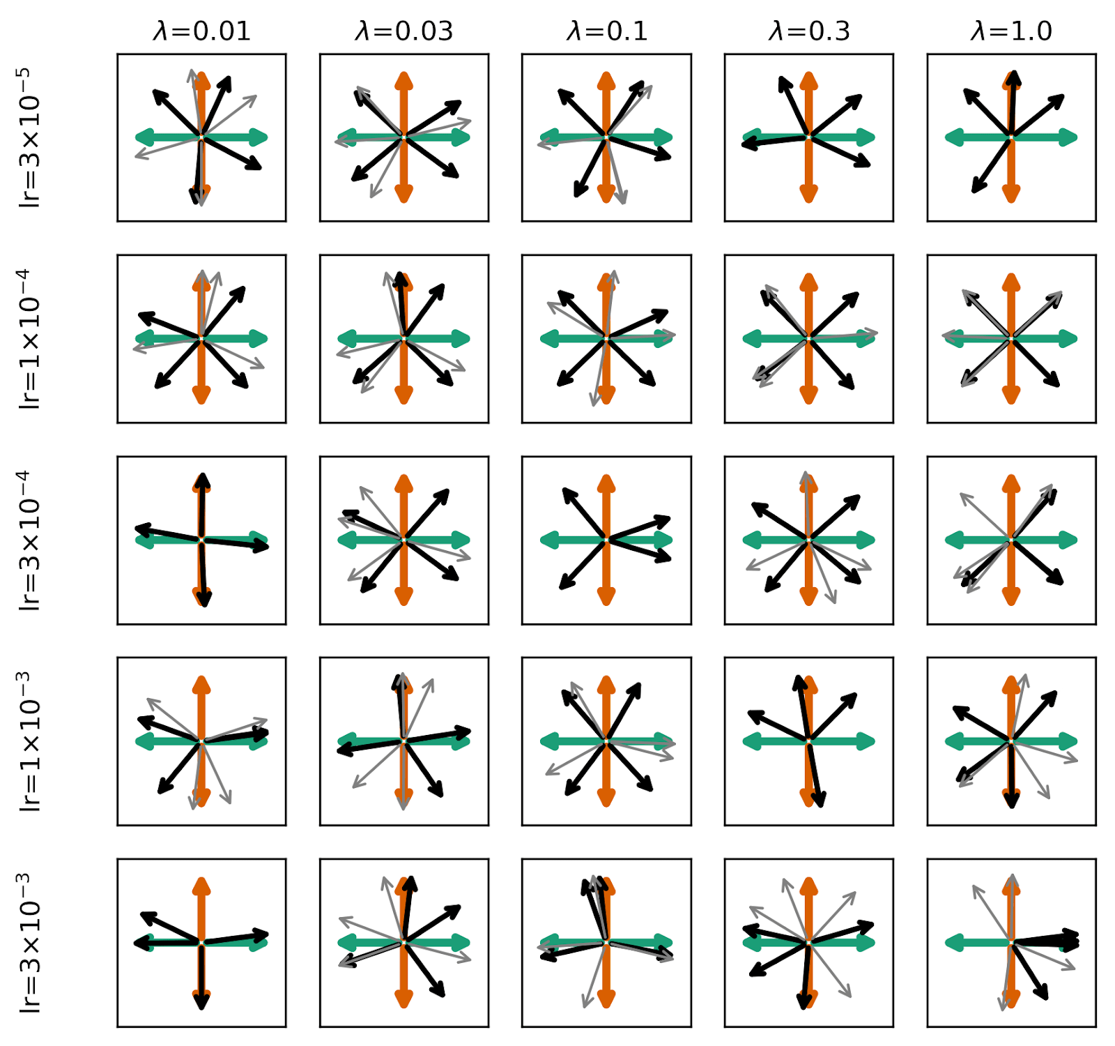
Can this effect, where the model learns composed pairs of features, be avoided simply through choosing better standard hyperparameters (learning rate and )? Probably not:
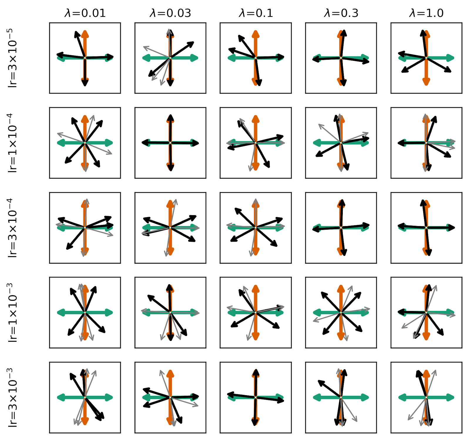
Uncorrelated Feature Amplitudes
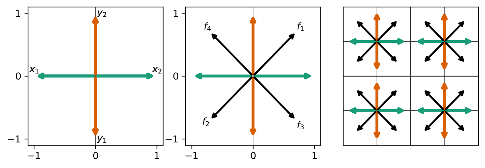
We next consider the case where the feature amplitudes within a given data vector are completely uncorrelated, with , so that and . Whereas in the previous problem, only four (arbitrarily scaled) data vectors could exist, now an infinite number of possible data vectors can be generated, but there still only exist two features in each set and therefore four total composed pairs.
We perform the same experiments as in the previous section, and replicate the same figures from the previous section below. Surprisingly, We find that the model more cleanly finds composed pairs than in the case where the input data vectors were pure composed pairs. By breaking the feature amplitude correlation, SAEs almost uniformly learn perfect composed pairs for all parameters studied. We note briefly that, in the grid below, some SAEs find monosemantic features at high learning rate and low (see the light grey arrows in the bottom left panels), but even when these monosemantic realizations are achieved, other realizations of the autoencoder find lower loss, polysemantic realizations with composed pairs.
Does a Cosine Similarity Loss Term Fix This Problem?
In Do sparse autoencoders find "true features"? [LW · GW], a possible solution to this problem is proposed:
I propose including an additional regularisation term in the SAE loss to penalise geometric non-orthogonality of the feature directions discovered by the SAE. One way to formalise this loss could be as the sum of the absolute values of the cosine similarities between each pair of feature directions discovered in the activation space. Neel Nanda's findings here suggest that the decoder rather than the encoder weights are more likely to align with the feature direction as the encoder's goal is to detect the feature activations, which may involve compensating for interference with other features.
We tried this, and for our small model it doesn’t help.
We calculated the cosine similarity between each column of the decoder weight matrix, , and stored those cosine similarity values in the square matrix , where is the hidden dimension size of the SAE. is symmetric, so we only need to consider the lower triangular part (denoted tril()). We tried adding two variations of an -based term to the loss function:
- coeff * mean(tril())
- coeff * mean(abs(tril())
Neither formulation improved the ability of our autoencoders to find monosemantic features.
- In the first case (no abs() on ), we found that the models found the same solution as above. This makes sense! The four features that we find above are in a minimal cosine-sim configuration, it’s just rotated compared to what we want, and this -based term doesn’t say anything about the orientation of features in activation space, just their distance from one another.
- For the second case (with abs() on ), we found either the same solution, or a solution where some feature decoder vectors collapsed (see below). This occurs because we normalize the decoder weights at each timestep, and it’s more favorable to have two features be aligned ( = 1) than it is to rotate a (magnitude 1) feature around to a more useful part of activation space.
- For example, consider the case where we have two vectors that are aligned, and two vectors that are perpendicular, like in 3 of the panels in the figure below. One of the two aligned vectors has an angle of 0, 90 , and 90 with the other vectors (cosine sims = 1, 0, 0). Rotating one of the aligned features to a more useful position requires it to pass through a spot where the angle between it and the three other features are 45, 45, and 135 (cosine sims = , , and ). If we sum up the absolute values of the cosine sim, this rotated vector has a higher abs(cos-sim): 1 < , so the vectors stay collapsed and it doesn’t rotate around to a more useful location in activation space.
Just because this additional loss term did not help this small toy context does not mean that it couldn’t help find more monosemantic features in other models! We find that it doesn’t fix this very specific case, but more tests are needed.
What if the SAE Actually Gets to See the True Features?
In the experiments I discussed above, every data vector is two-hot, and an and always co-occur. What if we allow data vectors to be one-hot (only containing one of OR ) with some probability ? We sample composed data vectors with probability . We tried this for and while SAEs are more likely to find the true features, it’s still not a sure thing – even when compositions occur only 25% of the time and feature amplitudes are completely uncorrelated in magnitude!
Below we repeat our toy model and SAE plots for the case where . Certainly more SAEs find true features in the lowest-loss instance whereas with , none did. But there’s no robust trend in learning rate and .
Takeaways
- Features in natural datasets can be composed, occurring in combination with other features. We can model this with synthetic data vectors and toy models.
- Small toy models store composed feature sets using superposition.
- Sparse autoencoders (SAEs) trained on these composed feature sets can find composed features rather than the true underlying features due to the penalty in their loss function.
- This happens even when the SAEs get to see the true features 75% of the time!
- We should consider how to train SAEs that aren’t susceptible to this failure mode.
- Strangely, this effect is worse when the composed pairs are less prominent in the input data (uncorrelated amplitude case) than it is in the case where the input data is always made up of these composed pairs.
Future work
This post only scratched the surface of the exploration work that we want to do with these toy models. Below are some experiments and ideas that we’re excited to explore:
- The 2-sets-of-2-features case is really special. For two sets each of features, the number of possible composed pairs is while the number of total features is just . These are both 4 in our case (although the individual features occur once every other data vector while the composed pairs occur once every four data vectors).
- As grows, composed pairs become increasingly sparse compared to the true underlying features, and we expect SAEs to recover the true features when each of the composed pairs are sparse. We’re interested in understanding how sparse (or not!) a composed pair needs to be compared to the underlying true features to make a model switch between learning composed pairs and true features.
- In the limit where is large, we expect SAEs to learn true features and not composed pairs. But what if two specific features e.g., are very highly correlated (so that rarely occurs with any other than and vice-versa)?
- What if we use a different probability distribution so that frequency follows something interesting like Zipf’s law?
- What happens as superposition becomes messier than antipodal pairs? Here we studied a case where the hidden model dimension is half the length of the feature vector. What if we have 10 total features and the hidden dimension is 3 or 4?
- What happens if we have more than two sets of composed features?
- How can we engineer SAEs to learn the underlying features rather than the composed pairs?
- Can perfect SAEs be created using “simple” tweaks? E.g., adding terms to the loss or tweaking hyperparameters?
- Is it essential to have some understanding of the training data distribution or the distribution of features in the dataset? How do SAEs perform for different types of feature distributions and how does the feature distribution affect the efficacy of engineering improvements?
- It feels like it shouldn’t be too hard to come up with something that makes perfect SAEs for the 2-sets-of-2-features case we studied here. If we find something in these small models, does it generalize?
We may not have time to get around to working on all of these questions, but we hope to work on some of them. If you’re interested in pursuing these ideas with us, we’d be happy to collaborate!
Code
The code used to produce the analysis and plots from this post is available online in https://github.com/evanhanders/superposition-geometry-toys . See in particular https://github.com/evanhanders/superposition-geometry-toys/blob/main/experiment_2_hid_dim.ipynb .
Acknowledgments
We’re grateful to Esben Kran, Adam Jermyn, and Joseph Bloom for useful comments which improved the quality of this post. We’re grateful to Callum McDougall and the ARENA curriculum for providing guidance in setting up and training SAEs in toy models and to Joseph Bloom for his https://github.com/jbloomAus/mats_sae_training repository which helped us set up our SAE class. We thank Adam Jermyn and Joseph Bloom for useful discussions while working through this project. EA Thanks Neel Nanda for a really useful conversation that led him to this idea at EAG in February.
Funding: EA and JH are KITP Postdoctoral Fellows, so this research was supported in part by NSF grants PHY-2309135 and PHY-1748958 to the Kavli Institute for Theoretical Physics (KITP) and by the Gordon and Betty Moore Foundation through Grant No. GBMF7392.
Citing this post
@misc{anders_etal_2024_composedtoymodels_2d,
   title = { Sparse autoencoders find composed features in small toy models  },
   author = {Anders, Evan AND Neo, Clement AND Hoelscher-Obermaier, Jason AND Howard, Jessica N.},
   year = {2024},
   howpublished = {\url{https://www.lesswrong.com/posts/a5wwqza2cY3W7L9cj/sparse-autoencoders-find-composed-features-in-small-toy}},
}- ^
But note that here I’m defining sparsity as occurrence frequency. Probably there’s a truer notion of sparsity and in that notion these data are probably sparse.
- ^
Though note that this is slightly different from Anthropic’s suggestion in the February update, where they chose to normalize their vectors so that each data point in the activations has a variance of 1. I think if you use the mean squared error compared to the squared error, this becomes equivalent to what I did here, but I’m not 100% sure.
12 comments
Comments sorted by top scores.
comment by Ali Shehper (ali-shehper) · 2024-03-18T22:53:43.471Z · LW(p) · GW(p)
Hey guys, great post and great work!
I have a comment, though. For concreteness, let me focus on the case of (x_2, y_1) composition of features. This corresponds to feature vectors of the form A[0, 1, 1, 0] in the case of correlated feature amplitudes and [0, a, b, 0] in the case of uncorrelated feature amplitudes. Note that the plane spanned by x_2 and y_1 admits an infinite family of orthogonal bases; one of which, for example, is [0, 1, 1, 0] and [0, 1, -1, 0]. When we train a Toy Model of Superposition, we plot the projection of our choice of feature basis as done by Anthropic and also by you guys. However, the training dataset for the SAE (that you trained afterward) contains no information about the original (arbitrarily chosen by us) basis. SAEs could learn to decompose vectors from the dataset in terms of *any* of the infinite family of bases.
This is exactly what some of your SAEs seem to be doing. They are still learning four antipodal directions (which are just not the same as the four antipodal directions corresponding to your original chosen basis). This, to me, seems like a success of the SAE.
We should not expect the SAE to learn anything about the original choice of basis at all. This choice of basis is not part of the SAE training data. If we want to be sure of this, we can plot the training data of the SAE on the plane (in terms of a scatter plot) and see that it is independent of any choice of bases.
↑ comment by LawrenceC (LawChan) · 2024-04-27T01:52:02.841Z · LW(p) · GW(p)
It's actually worse than what you say -- the first two datasets studied here have privileged basis 45 degrees off from the standard one, which is why the SAEs seem to continue learning the same 45 degree off features. Unpacking this sentence a bit: it turns out that both datasets have principle components 45 degrees off from the basis the authors present as natural, and so as SAE in a sense are trying to capture the principle directions of variation in the activation space, they will also naturally use features 45 degrees off from the "natural" basis.
Consider the first example -- by construction, since x_1 and x_2 are anticorrelated perfectly, as are y_1 and y_2, the data is 2 dimensional and can be represented as x = x_1 - x_2 and y = y_1 - y_2. Indeed, this this is exactly what their diagram is assuming. But here, x and y have the same absolute magnitude by construction, and so the dataset lies entirely on the diagonals of the unit square, and the principal components are obviously the diagonals.
Now, why does the SAE want to learn the principle components? This is because it allows the SAE to have smaller activations on average for a given weight norm.
Consider the representation that is axis aligned, in that the SAE neurons are x_1, x_2, y_1, y_2 -- since there's weight decay, the encoding and decoding weights want to be of the same magnitude. Let's suppose that the encoding and decoding weights are of size s. Now, if the features are axis aligned, the total size of the activations will be 2A/s^2. But if you instead use the neurons aligned with x_1 + y_1, x_1 + y_2, x_2 + y_1, x_2 + y_2, the activations only need to be of size \sqrt 2 A/s^2. This means that a non-axis aligned representation will have lower loss. Indeed, something like this story is why we expect the L1 penalty to recover "true features" in the first place.
The story for the second dataset is pretty similar to the first -- when the data is uniformly distributed over a unit square, the principle directions are the diagonals of the square, not the standard basis.
Replies from: evan-anders↑ comment by Evan Anders (evan-anders) · 2024-04-29T16:24:05.725Z · LW(p) · GW(p)
Hi Lawrence! Thanks so much for this comment and for spelling out (with the math) where and how our thinking and dataset construction were poorly setup. I agree with your analysis and critiques of the first dataset. The biggest problem with that dataset in my eyes (as you point out): the true actual features in the data are not the ones that I wanted them to be (and claimed them to be), so the SAE isn't really learning "composed features."
In retrospect, I wish I had just skipped onto the second dataset which had a result that was (to me) surprising at the time of the post. But there I hadn't thought about looking at the PCs in hidden space, and didn't realize those were the diagonals. This makes a lot of sense, and now I understand much better why the SAE recovers those.
My big takeaway from this whole post is: I need to think on this all a lot more! I've struggled a lot to construct a dataset that successfully has some of the interesting characteristics of language model data and also has interesting compositions / correlations. After a month of playing around and reflection, I don't think the "two sets of one-hot features" thing we did here is the best way to study this kind of phenomenon.
↑ comment by Evan Anders (evan-anders) · 2024-03-20T17:01:26.198Z · LW(p) · GW(p)
Thanks for the comment! Just to check that I understand what you're saying here:
We should not expect the SAE to learn anything about the original choice of basis at all. This choice of basis is not part of the SAE training data. If we want to be sure of this, we can plot the training data of the SAE on the plane (in terms of a scatter plot) and see that it is independent of any choice of bases.
Basically -- you're saying that in the hidden plane of the model, data points are just scattered throughout the area of the unit circle (in the uncorrelated case) and in the case of one set of features they're just scattered within one quadrant of the unit circle, right? And those are the things that are being fed into the SAE as input, so from that perspective perhaps it makes sense that the uncorrelated case learns the 45 angle vectors, because that's the mean of all of the input training data to the SAE. Neat, hadn't thought about it in those terms.
This, to me, seems like a success of the SAE.
I can understand this lens! I guess I'm considering this a failure mode because I'm assuming that what we want SAEs to do is to reconstruct the known underlying features, since we (the interp community) are trying to use them to find the "true" underlying features in e.g., natural language. I'll have to think on this a bit more. To your point -- maybe they can't learn about the original basis choice, and I think that would maybe be bad?
Replies from: ali-shehper↑ comment by Ali Shehper (ali-shehper) · 2024-03-25T03:29:11.547Z · LW(p) · GW(p)
Hi Evan, thank you for the explanation, and sorry for the late reply.
I think that the inability to learn the original basis is tied to the properties of the SAE training dataset (and won't be solved by supplementing SAEs with additional terms in its loss function). I think it's because we could have generated the same dataset with a different choice of basis (though I haven't tried formalizing the argument nor run any experiments).
I also want to say that perhaps not being able to learn the original basis is not so bad after all. As long as we can represent the full number of orthogonal feature directions (4 in your example), we are okay. (Though this is a point I need to think more about in the case of large language models.)
If I understood Demian Till's post right, his examples involved some of the features not being learned at all. In your example, it would be equivalent to saying that an SAE could learn only 3 feature directions and not the 4th. But your SAE could learn all four directions.
Replies from: evan-anders↑ comment by Evan Anders (evan-anders) · 2024-03-28T17:08:44.047Z · LW(p) · GW(p)
Hi Ali, sorry for my slow response, too! Needed to think on it for a bit.
- Yep, you could definitely generate the dataset with a different basis (e.g., [1,0,0,0] = 0.5*[1,0,1,0] + 0.5*[1,0,-1,0]).
- I think in the context of language models, learning a different basis is a problem. I assume that, there, things aren't so clean as "you can get back the original features by adding 1/2 of that and 1/2 of this". I'd imagine it's more like feature1 = "the in context A", feature 2 = "the in context B", feature 3 = "the in context C". And if the is a real feature (I'm not sure it is), then I don't know how to back out the real basis from those three features. But I think this points to just needing to carry out more work on this, especially in experiments with more (and more complex) features!
- Yes, good point, I think that Demian's post was worried about some features not being learned at all, while here all features were learned -- even if they were rotated -- so that is promising!
↑ comment by Demian Till · 2024-04-04T11:30:50.093Z · LW(p) · GW(p)
Regarding some features not being learnt at all, I was anticipating this might happen when some features activate much more rarely than others, potentially incentivising SAEs to learn more common combinations instead of some of the rarer features. In order to potentially see this we'd need to experiment with more variations as mentioned in my other comment
comment by Demian Till · 2024-04-04T11:12:19.122Z · LW(p) · GW(p)
Nice work! I was actually planning on doing something along these lines and still have some things I'd like to try.
Interestingly your SAEs appear to be generally failing to even find optimal solutions w.r.t the training objective. For example in your first experiment with perfectly correlated features I think the optimal solution in terms of reconstruction loss and L1 loss combined (regardless of the choice of the L1 loss weighting) would have the learnt feature directions (decoder weights) pointing perfectly diagonally. It looks like very few of your hyperparameter combinations even came close to this solution.
My post was concerned primarily with the training objective being misaligned with what we really want, but here we're seeing an additional problem of SAEs struggling to even optimise for the training objective. I'm wondering though if this might be largely/entirely a result of the extremely low dimensionality and therefore very few parameters causing them to get stuck in local minima. I'm interested to see what happens with more dimensions and more variation in terms of true feature frequency, true feature correlations, and dictionary size. And orthogonality loss may have more impact in some of those cases.
Replies from: evan-anders↑ comment by Evan Anders (evan-anders) · 2024-04-11T23:47:51.321Z · LW(p) · GW(p)
Hi Demian! Sorry for the really slow response.
Yes! I agree that I was surprised that the decoder weights weren't pointing diagonally in the case where feature occurrences were perfectly correlated. I'm not sure I really grok why this is the case. The models do learn a feature basis that can describe any of the (four) data points that can be passed into the model, but it doesn't seem optimal either for L1 or MSE.
And -- yeah, I think this is an extremely pathological case. Preliminary results look like larger dictionaries finding larger sets of features do a better job of not getting stuck in these weird local minima, and the possible number of interesting experiments here (varying frequency, varying SAE size, varying which things are correlated) is making for a pretty large exploration space.
comment by Logan Riggs (elriggs) · 2024-03-20T22:09:18.344Z · LW(p) · GW(p)
Hey! Thanks for doing this research.
Lee Sharkey et al did a similar experiment [LW · GW] a while back w/ much larger number of features & dimensions, & there were hyperaparameters that perfectly reconstructed the original dataset (this was as you predicted as N increases).
Hoagy still hosts a version of our replication here (though I haven't looked at that code in a year!).
Replies from: evan-anders↑ comment by Evan Anders (evan-anders) · 2024-03-21T18:00:07.764Z · LW(p) · GW(p)
Hi Logan! Thanks for pointing me towards that post -- I've been meaning to get around to reading it in detail and just finally did. Glad to see that the large-N limit seems to get perfect reconstruction for at least one similar toy experiment! And thanks for sharing the replication code.
I'm particularly keen to learn a bit more about the correlated features -- did you (or do you know of anyone) who has studied toy models where they have a few features that are REALLY correlated with one another, and that basically never appear with other features? I'm wondering if such features could bring back the problem that we saw here, even in a very high-dimensional model / dataset. Most of the metrics in that post are averaged over all features, so don't really differentiate between correlated or not, etc.
Replies from: elriggs↑ comment by Logan Riggs (elriggs) · 2024-03-22T04:17:42.705Z · LW(p) · GW(p)
Agreed. You would need to change the correlation code to hardcode feature correlations, then you can zoom in on those two features when doing the max cosine sim.