Faithful vs Interpretable Sparse Autoencoder Evals
post by Louka Ewington-Pitsos (louka-ewington-pitsos) · 2024-07-12T05:37:18.525Z · LW · GW · 0 commentsContents
  Summary
  Faithfullness vs Interpretability
  Explainability vs Interpretability
  Popular Metrics
    Formalization
    Measures of Interpretability
      L1
        Description
        Usage
        Advantages
        Disadvantages
      L0
        Description
        Usage
        Advantages
        Disadvantages
      Probe Loss[7][3]
        Description
        Purpose
        Advantages
        Disadvantages
      Activation Prediction Loss[3][8]
        Description
        Purpose
        Advantages
        Disadvantages
      Human Analysis[1]
        Description
        Purpose
        Advantages
        Disadvantages
    Measures of Faithfulness
      MSE Reconstruction
        Description
        Purpose
        Advantages
        Disadvantages
      Downstream Reconstruction[9]
        Description
        Purpose
        Advantages
        Disadvantages
      Downstream Loss[9][3]
        Description
        Purpose
        Advantages
        Disadvantages
  What about Universality?
  Conclusion
None
No comments
Summary
Sparse Autoencoders (SAEs) have become a popular tool in Mechanistic Interpretability but at the time of writing there is no standardm automated way to accurately assess the quality of a SAE. In practice many different metrics are applied and interpreted to assess SAE quality in different studies.
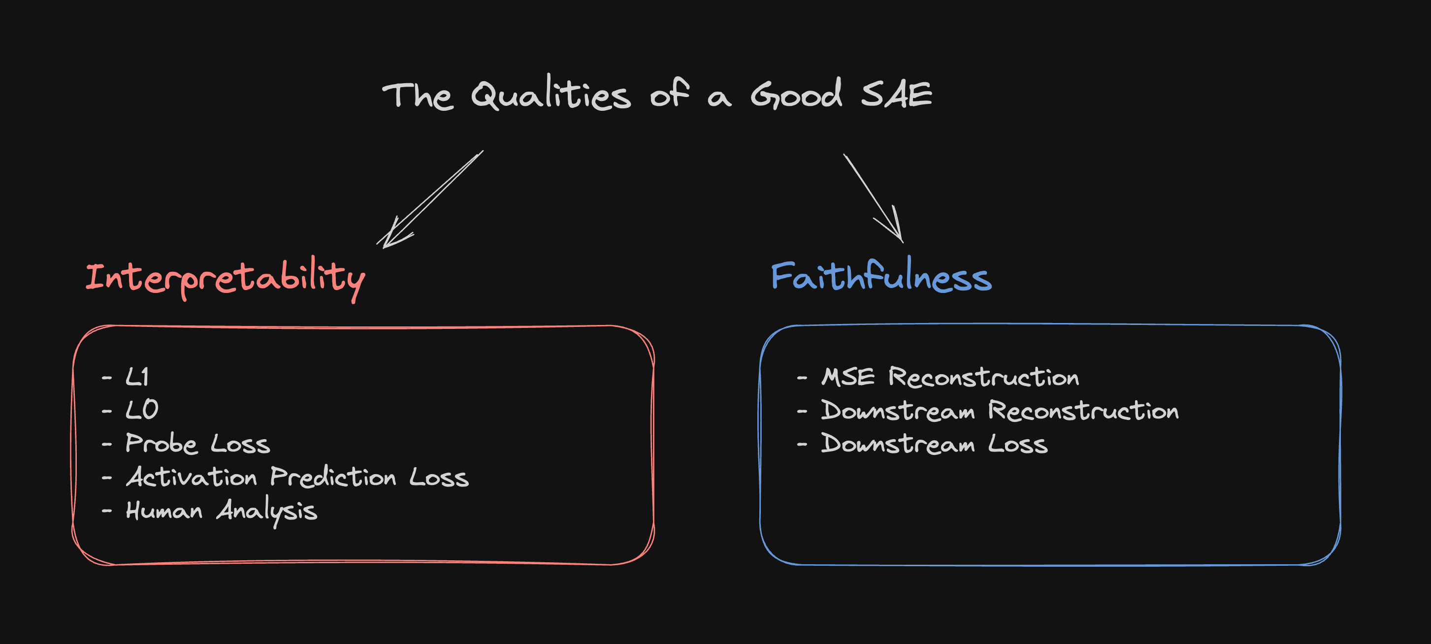
Conceptually however what makes a good SAE is relatively uncontroversial: its latent features must reflect the structure of the model it was trained on whilst also reflecting the structure of human linguistic understanding[1][2][3]. These twin objectives are usually referred to as "Faithfulness" and "Interpretability"[1][4].
In this article we will go through 8 common metrics used to evaluate the quality of a SAE and try to demonstrate that, though this is sometimes not stated explicitly, each metric can be thought of as attempting to measure either Faithfulness or Interpretability.
This article is not an attempt to prove anything, but rather suggest a mental model which might be useful.
Faithfullness vs Interpretability
At this stage there is no widespread practical use for SAEs. When one arises a metric pertaining to this use will probably become the gold standard for what makes a "good" SAE.
Until then the qualities sought in an SAE are stated well by Huang et. al.[2]
A central goal of interpretability is to localize an abstract concept to a component of a deep learning model that is used during inference.
In other words a good SAE will be one which identifies "abstract concepts" in the linguistic sense and maps these to structures inside the host LM[1].
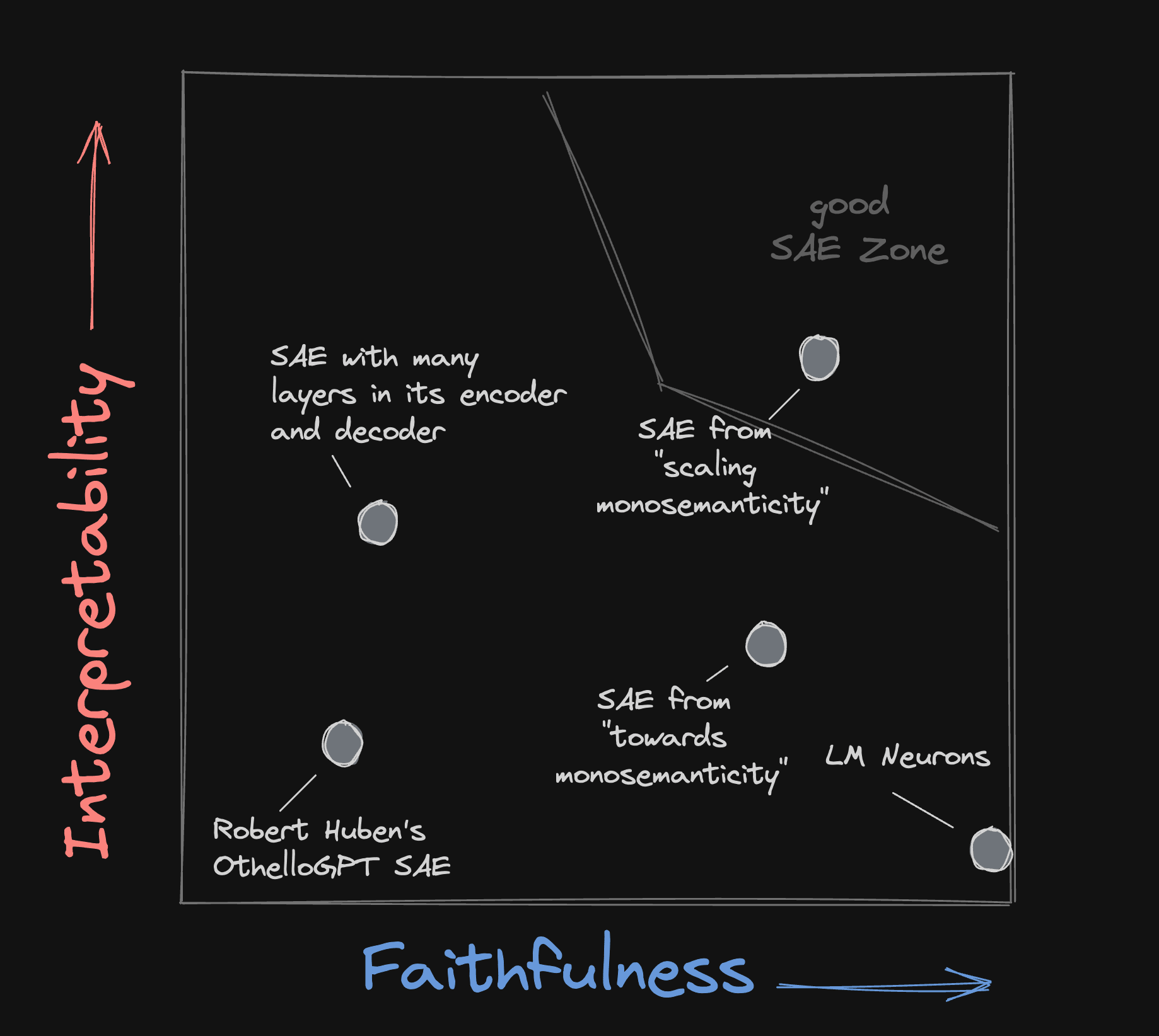
Importantly these two qualities are independent of one another. In fact to anyone who has trained a SAE the two will probably seem frustratingly opposed.
Interpretability can be achieved more easily by sacrificing the close relation held between the Autoencoder and the host model. For example by adding layers to the encoder and decoder pipelines.
Similarly Faithfullness can be achieved without interpretability. The most extreme example would be the neurons of the LM themselves, which are notoriously difficult to interpret[1]. A less extreme example would be an Autoencoder trained without any, or a very low sparsity loss term.
The goal of much of the current SAE literature is training one which achieves both Faithfullness and Interpretability at the same time.
Explainability vs Interpretability
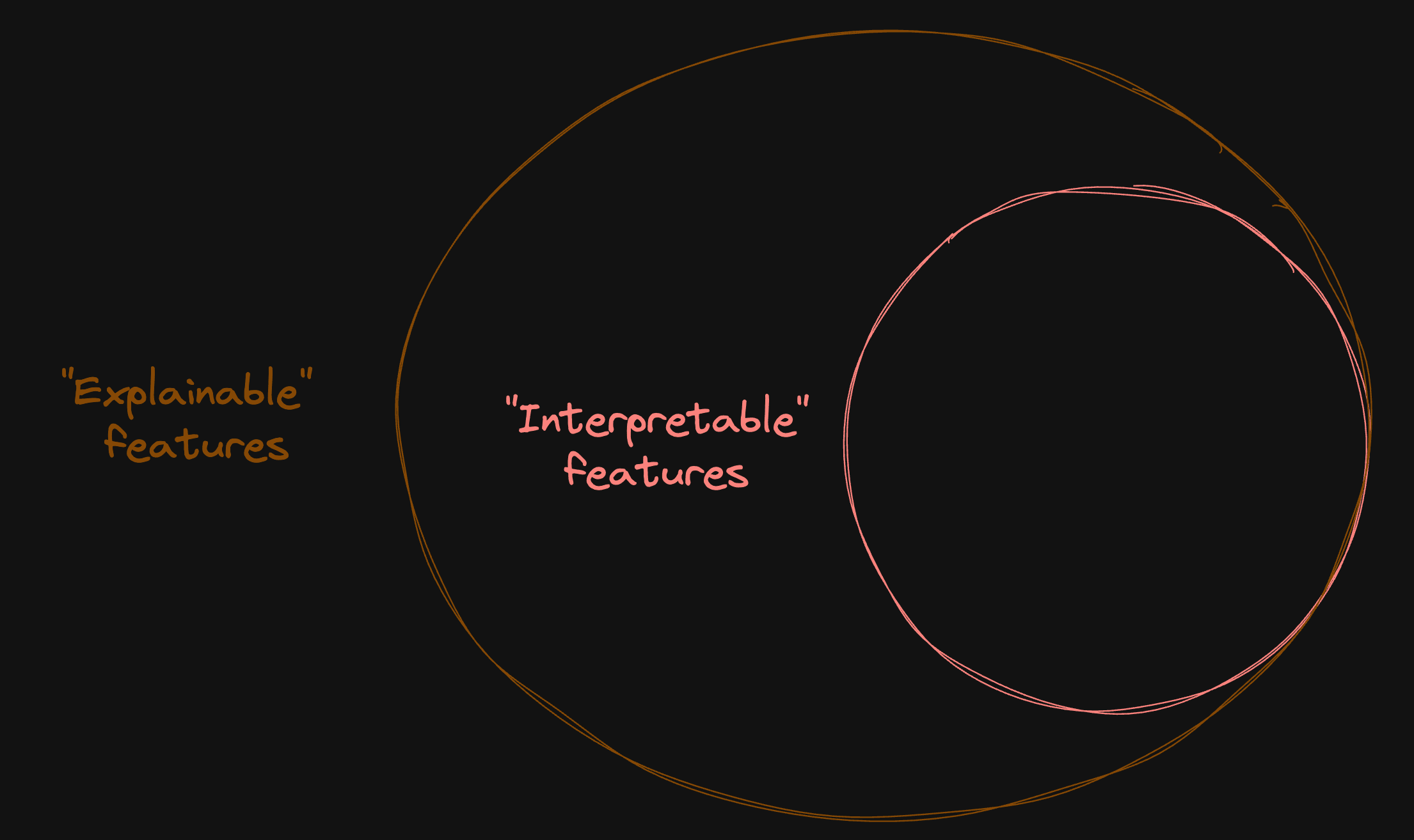
Importantly in the sense we are using it here "Interpretability" has a slightly broader meaning than its literal definition. We are expanding it to refer to a general correspondence with human understanding of language and thought.
The term Explainability as it is used in the literature has a narrower definition. It refers to any phenomena of a SAE which can be understood by a human[3][1]. Under this definition the ideal SAE must be more than merely perfectly Explainable. Features which fire with perfect accuracy on single words are highly Explainable but if these kinds of features make up the entire SAE it probably isn't going to be useful for anything.
Instead we want a SAE whose features are also interesting to humans and generally allow them to communicate with (e.g. steer) and understand LMs in ways that they find useful. This more stringent requirement is what we mean when we use the word Interpretability in this article, though this is by no means a recommendation that others follow suit.
Popular Metrics
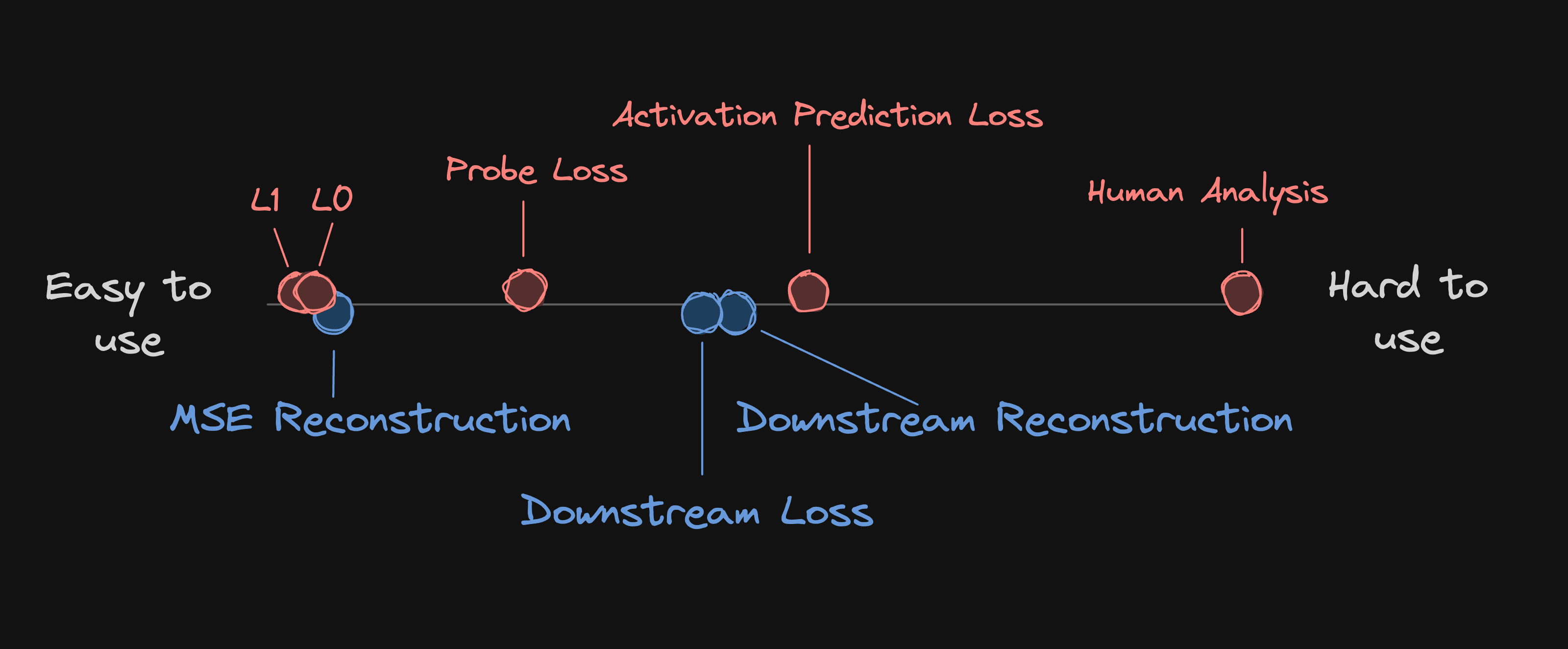
What follows is an enumeration of 8 metrics used in the SAE literature and their advantages and disadvantages as measures of Faithfulness and Interpretability. To give a quick overview we rank them below (very roughly) by how difficult they are to use in practice.
Formalization
Let be a Language Model.
Let be the 'th sample in an evaluation dataset containing total samples.
Let be the activations which flow out of a chosen transformer block of the residual stream of when the sample is fed into .
Let be a Sparse Autoencoder trained to take in , encode it into a latent representation of rank and then decode it back as close to again as possible using the same methods as Bricken et. al.[1]. Let be the actual output of after decoding. Let be just the encoder portion of such that . Let be the decoder portion such that .
Measures of Interpretability
L1
Description
The L1 norm for a single vector is the sum absolute values in a vector. In the context of SAEs the vector in question is the latent inside the Autoencoder. Geometrically L1 can be thought of as the "distance" between the vector and the origin.
Usually in the literature L1 refers to the average L1 over .
Usage
L1 is a key component of most sparse auto-encoder training pipelines. It is almost always the only component of the training loss which encourages sparsity in .
Advantages
- L1 is very cheap to calculate and easy to implement
- Though primarily used in the training loss, L1 gives some indication of Interpretability since if the L1 norm is very high there is a high likelihood that is not sparse, and in general latent features only start making sense to humans when is sparse[1].
Disadvantages
- In theory L1 can be deceptive as a measure of interpretability since a highly sparse vector with very high values wherever it is non-zero can still have a very high L1. Similarly L1 can be low of a vector with many non-zero values as long as all those values are low.
- As an unreliable measure of sparsity L1 can at best be considered a proxy for a proxy of Interpretability.
L0
Description
L0 is the count of non-zero elements in the latent vector . Mathematically:
Usage
In the literature L0, usually averaged across , is used as a direct measure of sparsity of the Autoencoder [5] and hence a very rough measure of interpretability or potential interpretability.
Advantages
- L0 is similarly very efficient to calculate and easy to implement in any language.
- L0 provides a direct measure of sparsity by counting the number of non-zero elements in the latent representation, making it a more accurate measure of Interpretability.
Disadvantages
- L0 is non-differentiable, meaning it cannot be used for training, though modified, differentiable versions of L0 do exist[6].
- Sparsity is still a very rough measure of Interpretability and so cannot be relied on on its own.
Probe Loss[7][3]
Description
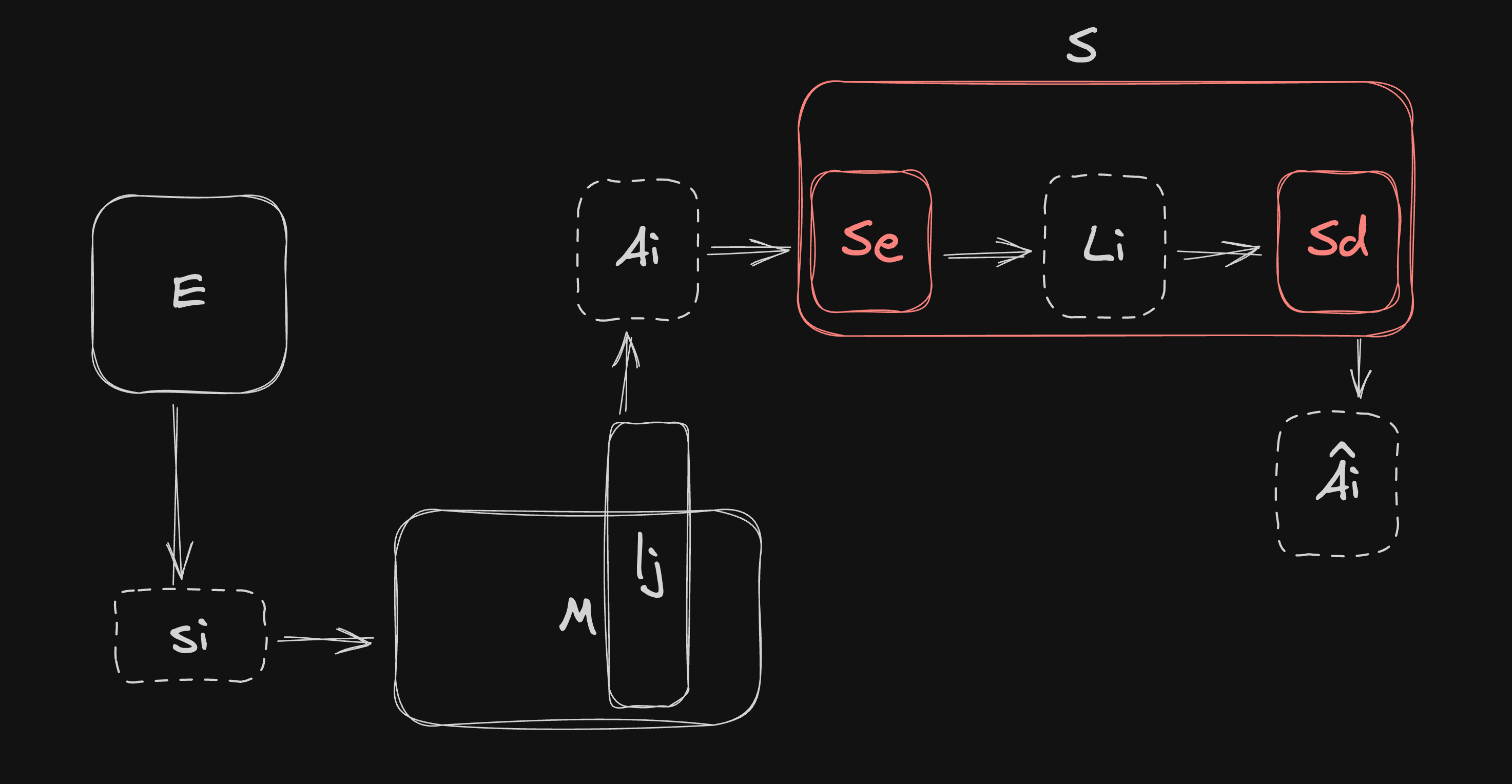
To calculate probe loss you first curate a binary classification dataset to reflect some concept such that it contains positive samples which exemplify that concept and also negative samples which do not. For instance the positive examples might contain positive sentiment and the negative ones neutral or negative sentiment.
Then when you want to assess your SAE you train a simple classifier, such as a logistic regression model to take the derived from a classification dataset sample as input and perform the classification. The Probe loss is simply the classification loss for that task.
More formally let the classification dataset be containing samples.
Let each sample from that dataset be where is the th input sample and is its ground truth label.
Let be a simple classifier which takes in the Autoencoder latent for the sample an returns a classification prediction. Let be a function which reads a sample into and returns the activations of block i.e. .
Let be some loss function such as Binary Cross EntropyL:
Let be the Probe Loss for that particular dataset.
Purpose
Probe Loss is named because of its relation to "Linear Probes". It has been used as a measure of Interpretability in Gao et. al.[3], where multiple classification datasets were created, most of them encoding high level concepts. However the same technique was used by Robert Huben as a measure of Faithfulness to determine whether a SAE could recover simple board state features from an OthelloGPT model[7]. In a very straightforward way Probe Loss gives us an idea of whether can be used to perform a particular kind of classification.
Advantages
- Probe Loss is very flexible and unlike the norms can be used to pinpoint the performance of the SAE on particular elements of human language, or elements of the host model .
- Probe Loss is also computationally cheap since the classifier must be small (ideally linear). A large classifier could learn the classification task on its own, which would invalidate it as a measure of the capabilities of .
Disadvantages
- For each capability you want to measure you must curate a new dataset which must be done with great care.
- Probe loss is not straightforward to implement, at least compared to calculating norms.
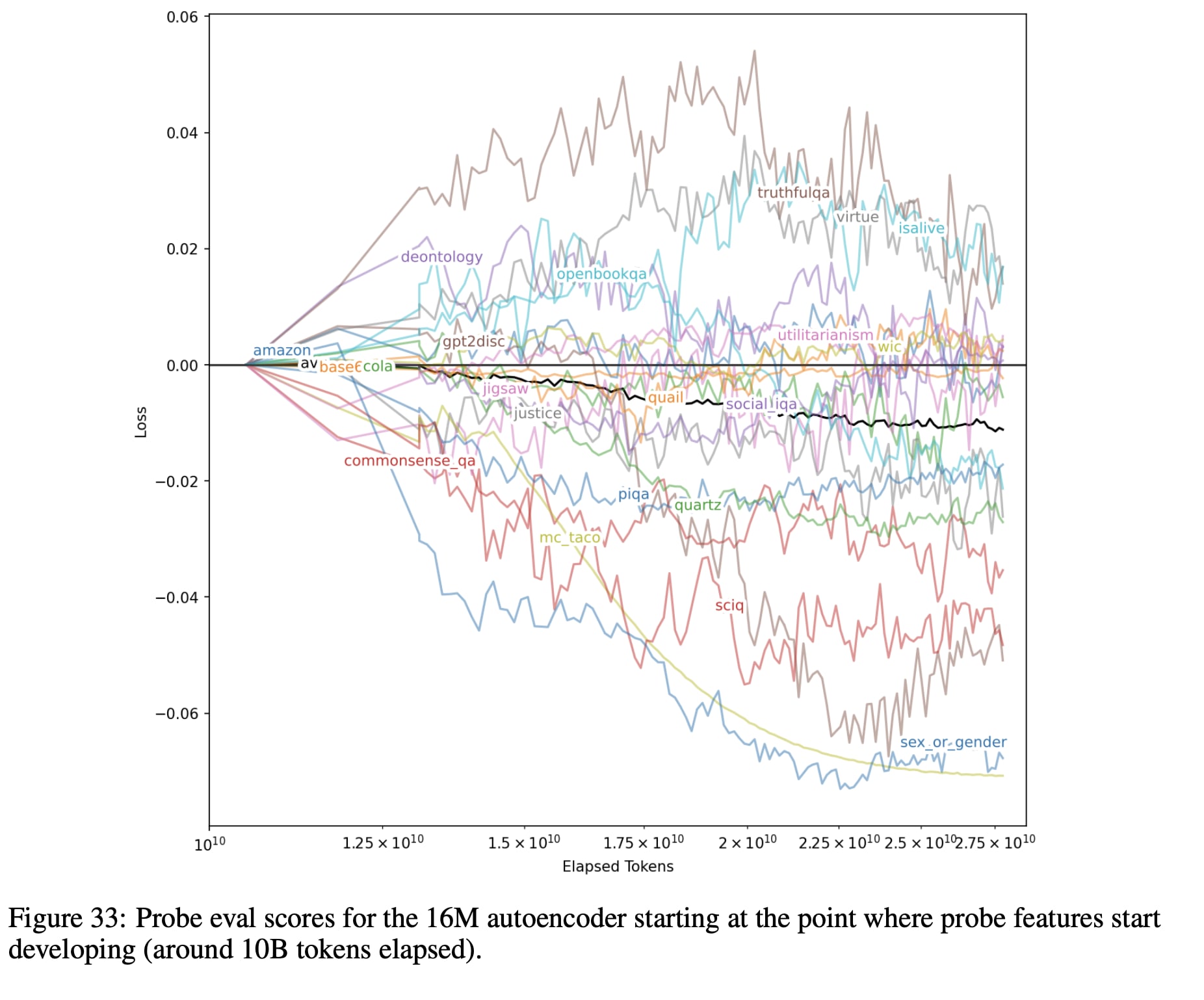
A SAE may have good Faithfulness and Interpretability while failing to facilitate any particular classification capability[7]. Therefore the loss on a single probe is likely not a good measure of overall SAE Interpretability or Faithfulness. Gao et. al.[3] found that even when averaging 61 Probes their Probe Loss was quite noisy, as can be seen in the figure below.
Taken from Gao et. al.[3]
Activation Prediction Loss[3][8]
Description
For each feature you wish to analyze:
- Select a set of examples which have high activations for that feature.
- Generate an "Explanation" of these examples. This could be as simple as passing them to a LM in a prompt and having the LM generate its best plaintext explanation of the underlying feature. Gao et. al.[3] took a different approach by generating explanations composed of what could be thought of as "phrase templates" which match all .
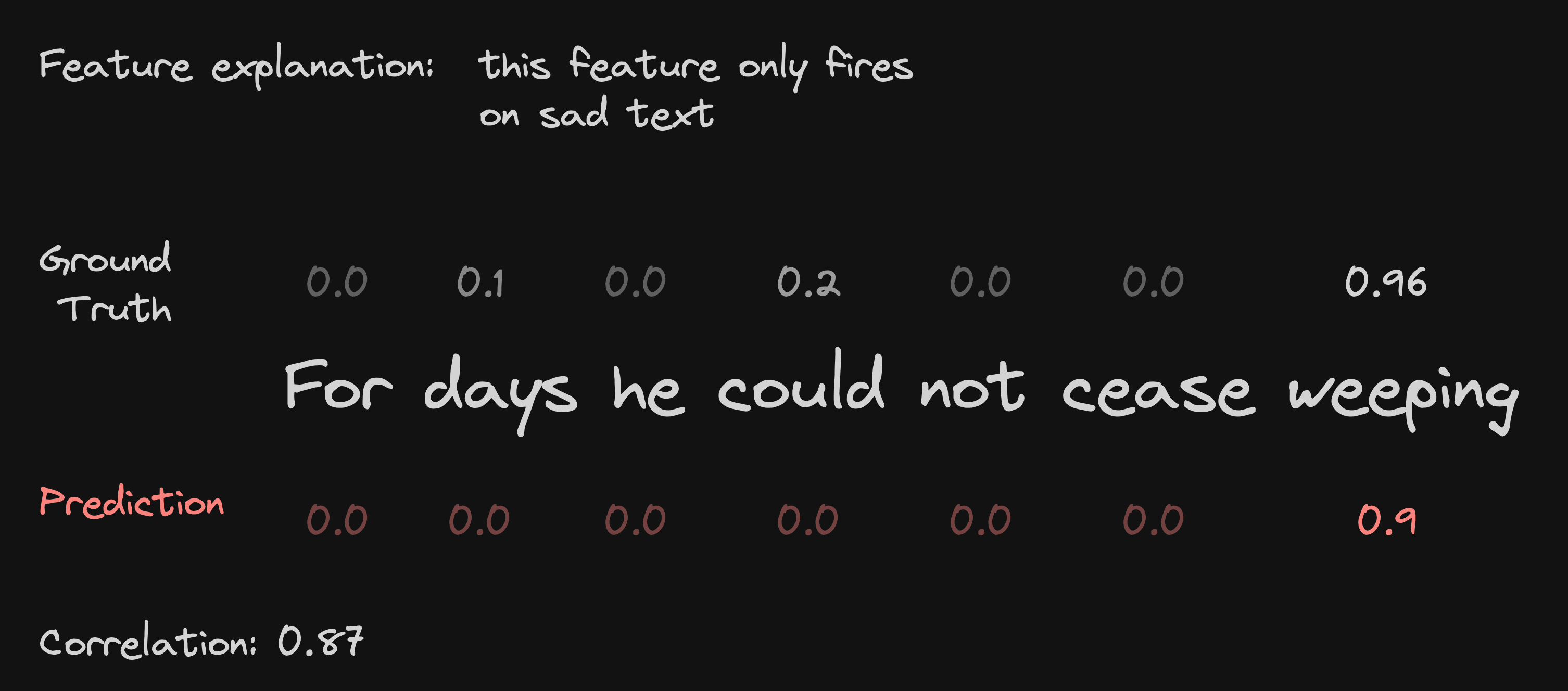
- Collect a new set of new evaluation examples. Let the full set of these evaluation examples be . These may be high activating examples for that feature or random examples (random samples will help avoid bias but you may need more of them to find any activations at all).
- Create a prediction function which uses the explanation to predict activations across , i.e. where is a sample from and are the predicted activations across that sample. For example, one could simply add and to a prompt which is then passed to a LM which then generates as a JSON sequence.
- Collect all and across and then use a measure of correlation between the real activations and the predicted activations such as spearman correlation to generate an overall Activation Prediction Loss for .
Now repeat this for each feature to get an overall Activation Prediction Loss.
Purpose
The idea behind Activation Prediction Loss is that features which cannot be predicted are likely to be random or nonsensical. Often the prediction function is a LM and is thought of as a proxy for human understanding, with the idea being that features which can be predicted accurately by humans are likely to be Explainable.
Advantages
- APL is a much more accurate measure of Interpretability than the norms and unlike Probe Loss it scores the features which actually do exist in rather than features which may or may not.
- The explanation can be useful in its own right, for instance for performing clustering or merely eyeballing the different kinds of features present in
Disadvantages
- APL can be very computationally expensive. If involves a LM then a whole prediction sequence must be generated times for every feature in , which is often millions of features.
- APL is not straightforward to implement
- APL can be prone to bias if great care is not put into the sampling of and the choice of loss function
- Very basic features like "token contains the letter A" are prone to scoring highly on APL while falling short of being interesting in terms of human understanding. For the purposes of assessing Interpretability APL might be seen as a "necessary but not sufficient" indicator.
Human Analysis[1]
Description
Create a human-readable "Interpretability" rubric, then for each feature calculate an Interpretability score by
- Selecting a set of examples which have high activations for that feature
- Having a human assessor apply the rubric given all examples to create a score for that feature
For instance in Bricken et. al.[1] the authors created a rubric which had the assessor read all the examples, form an interpretation for what the underlying feature was and then essentially rank how explainable and internally consistent the feature was.
Purpose
In Bricken et. al.[1] the rubric was only aimed at assessing Explainability but rubrics could be designed to assess Interpretability more generally.
Advantages
- Human Analysis is probably the gold standard when it comes to assessing the Interpretability of a SAE. Nothing is likely to give a better indication for whether a SAE corresponds to human understanding than having a human assess it.
Disadvantages
- Human Analysis is prohibitively expensive in most cases.
- Great care must be taken in designing the rubric and choosing samples to avoid bias or invalidation of the assessment.
Measures of Faithfulness
MSE Reconstruction
Description
In the context of SAEs MSE Reconstruction is the Mean Squared Error between the model activations for a particular sample and the Autoencoder reconstruction
Purpose
MSER is primarily used when training SAEs and it usually forms a major component of the loss function. The MSER loss term is designed to train the latent to be as close to a perfect compressed (or in the case of most SAEs, overcomplete and and sparse) representation of as possible.
Advantages
- MSER is very cheap to calculate and easy to implement.
- MSER is differentiable.
- MSER can serve as a rough proxy for how well the reflects the internal structure of since if the MSER is very high it means that the correspondence between and is likely to be small.
Disadvantages
We can imagine cases where an Autoencoder achieves a very low MSER, but fails to accurately represent in . For instance where is always very close to but the small differences turn out to be the most important component of from the perspective of .[9] Because of this MSER is at best a very rough a proxy of Faithfulness.
Downstream Reconstruction[9]
Description
Downstream Reconstruction is simply MSER taken between the activations at every block after (though in theory you could include as well), after we substitute the usual for the reconstructed in the forward pass of . It is calculated as follows:
Let have transformer blocks.
Let denote the activation of the th block in when is given the sample as input.
- Pass a sample into , recording all such that .
- Next we pass into a second time, pausing at .
- We then collect the activations which come out of and pass them into the Autoencoder to create the reconstruction .
- In a regular forward pass the next block would take in and things continue as normal. In this case we pass in instead (the details of what form is passed back in can differ from use case to use case).
- Continue the forward pass all the way to the end, recording an for each block after .
- Finally, take the MSE between every recorded pair of activations, this is your Downstream MSE Reconstruction loss for . Over the whole of we calculate as
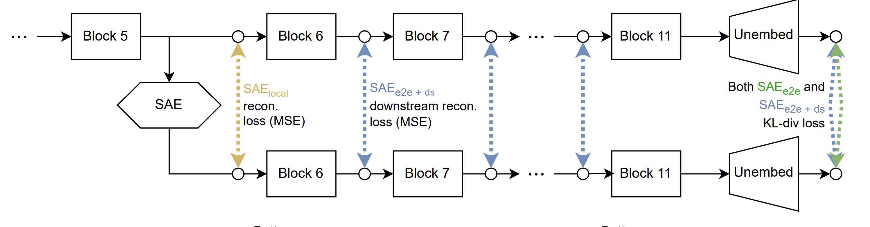
To add some visuals, the blue arrows in the diagram below collectively represent DR for a single sample as it was implemented in Braun et. al.[9]
Purpose
The Purpose of DR is to provide a version of MSER which is sensitive to downstream changes within the network, not just the immediate geometric difference between and
Advantages
- DR is differentiable, indeed it was primarily used for training in Braun et. al.[9]
- DR is a better measure of Faithfulness than MSER as must learn to reconstruct in such a way that the residual stream of the whole downstream model does not deviate much from what it would be normally. This will naturally force more information about the downstream of into
Disadvantages
- DR is more computationally expensive than MSER as each forward pass during training must pass through an additional transformer blocks and collect gradients.
Downstream Loss[9][3]
Description
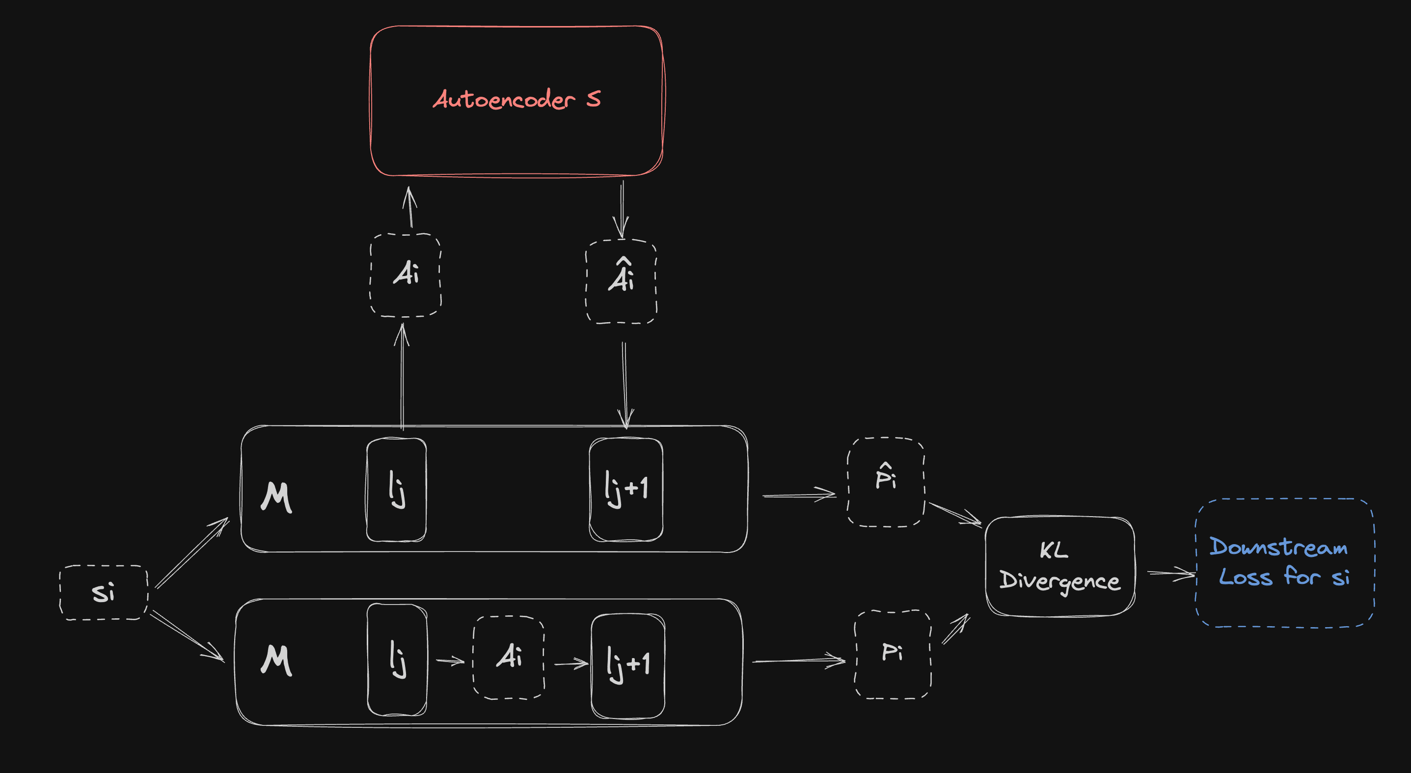
Downstream Loss is very similar to Downstream Reconstruction. The main difference is that it the loss is formed on the basis of the final token probabilities coming out of rather than intermediate activations. It is calculated as follows:
- Perform a forward pass as before, passing into . This time we discard the intermediate activations and instead record the the token logits which come out of (i.e. a score for each token in the vocabulary of ). These are then converted into token probabilities through a function like softmax.
- Next we perform a "reconstructed" forward pass as we did when calculating DR, i.e. passing into instead of but otherwise keeping all else the same. This time we end up with modified token logits which we convert to probabilities
- Finally, we calculate the Kullback-Leibler (KL) divergence (which essentially measures "how much information is lost") between the regular token probabilities and the ones based on : .
Repeat steps 1-7 as many times as you like on different samples and take the average KL divergence to arrive at Downstream Loss.
Purpose
The most common purpose of Downstream Loss is to identify "functionally important features" [9] i.e. those elements in which have an impact on what tokens end up coming out of .
Advantages
- Downstream Loss is likely an accurate indicator of Faithfulness since it shows how important the information lost between and is to the actual outputs coming out of . A very low Downstream Loss indicates that is probably very close to representing what is functionally important in .
- Downsteam loss is differentiable and can be used to train the SAE directly.
Disadvantages
- Like DR, Downstream Loss is somewhat computationally expensive, especially when is large since it requires a full forward pass through at each step. When used in training, gradients between and must also be stored.
- Downstream Loss is not trivial to implement
- Downstream Loss may be a less accurate measure of Faithfulness than Downstream Reconstruction as we can imagine a case where learns to make very similar to but uses very different circuits in than usual to do so. In such cases may fail to accurately reflect the structure of but still maintain a very low Downstream Loss.[9]
What about Universality?
Universality is another quality we would like our latent to achieve. is considered universal when its features remain Interpretable across many different corpuses and to many different humans (for instance humans who speak different languages) and when its features correspond to the internal structures of many different LMs, not just [1].
In this way we may think of there being two kinds of universality, Universal Interpretability and Universal Faithfulness. For instance, we can easily imagine training a SAE on a very limited corpus of Urdu technical jargon. Such a SAE would learn features which would not be Universally Interpretable (they would not seem to make sense to many humans) but could well be Universally Faithful (they may appear across many multilingual LMs).
Universality is certainly a quality we might want to achieve when training a SAE but we mention it here mainly to show that thinking about it through the lens of the two main objectives of Faithfulness and Interpretability is a reasonable thing to do.
Conclusion
It may be useful to conceptualize a good Sparse Autoencoder as one which maintains a close correspondence with the internal structure of its host model (Faithfulness) and with the structure of human language understanding (Interpretability).
While not always explicitly stated, many metrics used in practice to assess the quality of Sparse Autoencoders can be thought of as measuring one of these two qualities. Keeping this underlying dichotomy in mind may prove useful when assessing and explaining the outcomes of Sparse Autoencoder evaluations, especially to newcomers.
- ^
Trenton Bricken, Adly Templeton, Joshua Batson, Brian Chen, Adam Jermyn, Tom Conerly, Nick Turner, Cem Anil, Carson Denison, Amanda Askell, Robert Lasenby, Yifan Wu, Shauna Kravec, Nicholas Schiefer, Tim Maxwell, Nicholas Joseph, Zac Hatfield-Dodds, Alex Tamkin, Karina Nguyen, Brayden McLean, Josiah E Burke, Tristan Hume, Shan Carter, Tom Henighan, and Christopher Olah. Towards monosemanticity: Decomposing language models with dictionary learning. Transformer Circuits Thread, 2023. https://transformer-circuits.pub/2023/monosemanticfeatures/index.html
- ^
Jing Huang, Zhengxuan Wu, Christopher Potts, Mor Geva, Atticus Geiger. RAVEL: Evaluating Interpretability Methods on Disentangling Language Model Representations. arXiv preprint, 2024. URL https://arxiv.org/abs/2402.17700
- ^
Leo Gao, Tom Dupré la Tour, Henk Tillman, Gabriel Goh, Rajan Troll, Alec Radford, Ilya Sutskever, Jan Leike, Jeffrey Wu. Scaling and evaluating sparse autoencoders. arXiv preprint, 2024. URL https://doi.org/10.48550/arXiv.2406.04093
- ^
Daking Rai, Yilun Zhou, Shi Feng, Abulhair Saparov, Ziyu Yao. A Practical Review of Mechanistic Interpretability for Transformer-Based Language Models. arXiv preprint, 2024. URL https://doi.org/10.48550/arXiv.2407.02646
- ^
Joseph Bloom. Open Source Sparse Autoencoders for all Residual Stream Layers of GPT2-Small. LessWrong, 2024. URL https://www.lesswrong.com/posts/f9EgfLSurAiqRJySD/open-source-sparse-autoencoders-for-all-residual-stream [LW · GW]
- ^
Andrew Quaisley. Research Report: Alternative sparsity methods for sparse autoencoders with OthelloGPT. LessWrong, 2024. URL https://www.lesswrong.com/posts/ignCBxbqWWPYCdCCx/research-report-alternative-sparsity-methods-for-sparse [LW · GW]
- ^
Robert_AIZI. Research Report: Sparse Autoencoders find only 9/180 board state features in OthelloGPT. LessWrong, 2024. URL https://www.lesswrong.com/posts/arEub4eHo2EJfCHQX/research-report-sparse-autoencoders-find-only-9-180-board-state-features-in-othellogpt [LW · GW]
- ^
Steven Bills, Nick Cammarata, Dan Mossing, Henk Tillman, Leo Gao, Gabriel Goh, Ilya Sutskever, Jan Leike, Jeff Wu, and William Saunders. Language models can explain neurons in language models. OpenAI Blog, 2023. URL https://openaipublic.blob.core.windows.net/ neuron-explainer/paper/index.html
- ^
Dan Braun, Jordan Taylor, Nicholas Goldowsky-Dill, Lee Sharkey. Identifying Functionally Important Features with End-to-End Sparse Dictionary Learning. arXiv preprint, 2024. URL https://doi.org/10.48550/arXiv.2405.12241.
0 comments
Comments sorted by top scores.