Towards Multimodal Interpretability: Learning Sparse Interpretable Features in Vision Transformers

post by hugofry · 2024-04-29T20:57:35.127Z · LW · GW · 8 comments

Contents

  Executive Summary
  Motivation
  What is a Vision Transformer?
  What is CLIP?
  Training the SAE
  Examples of SAE Features
    Interesting and Amusing Features
      Era/Time Features:
        1950's Era Feature:
      Place/Culture Features:
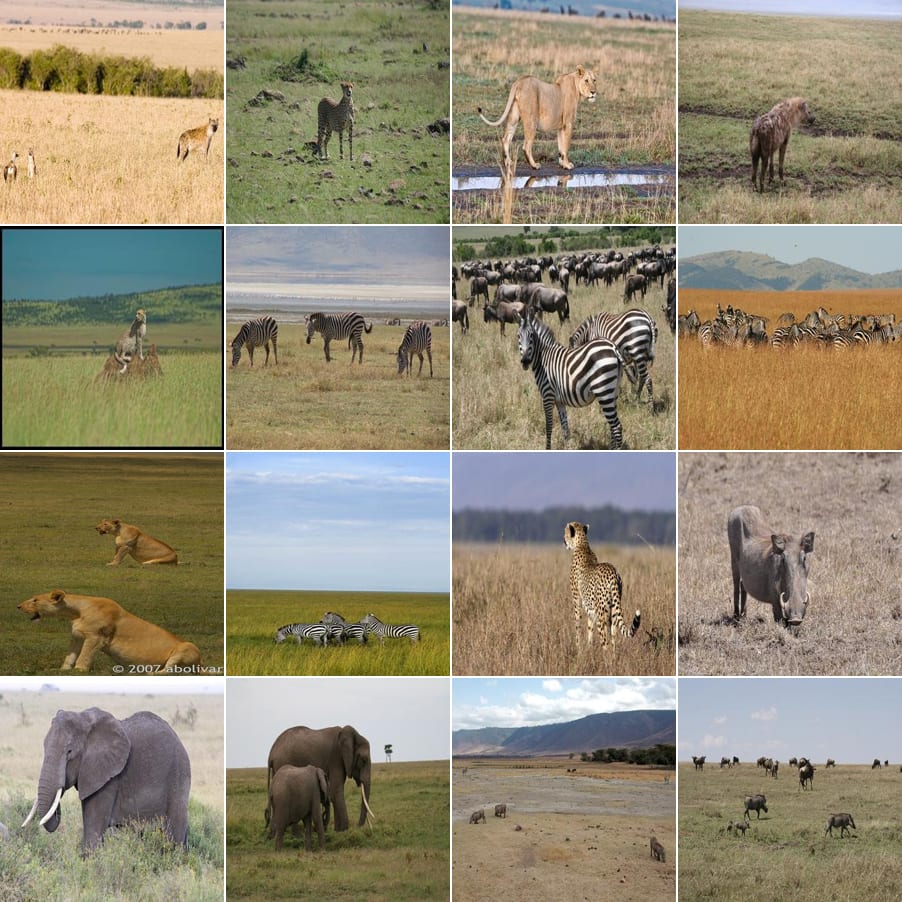
        African Animals:
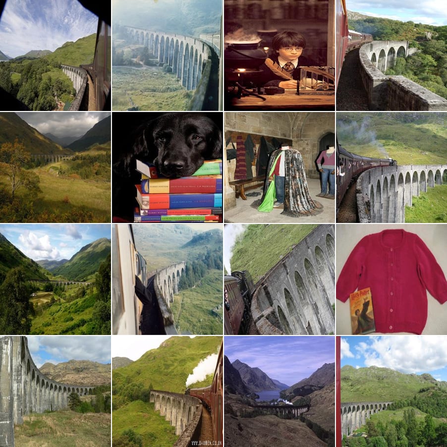
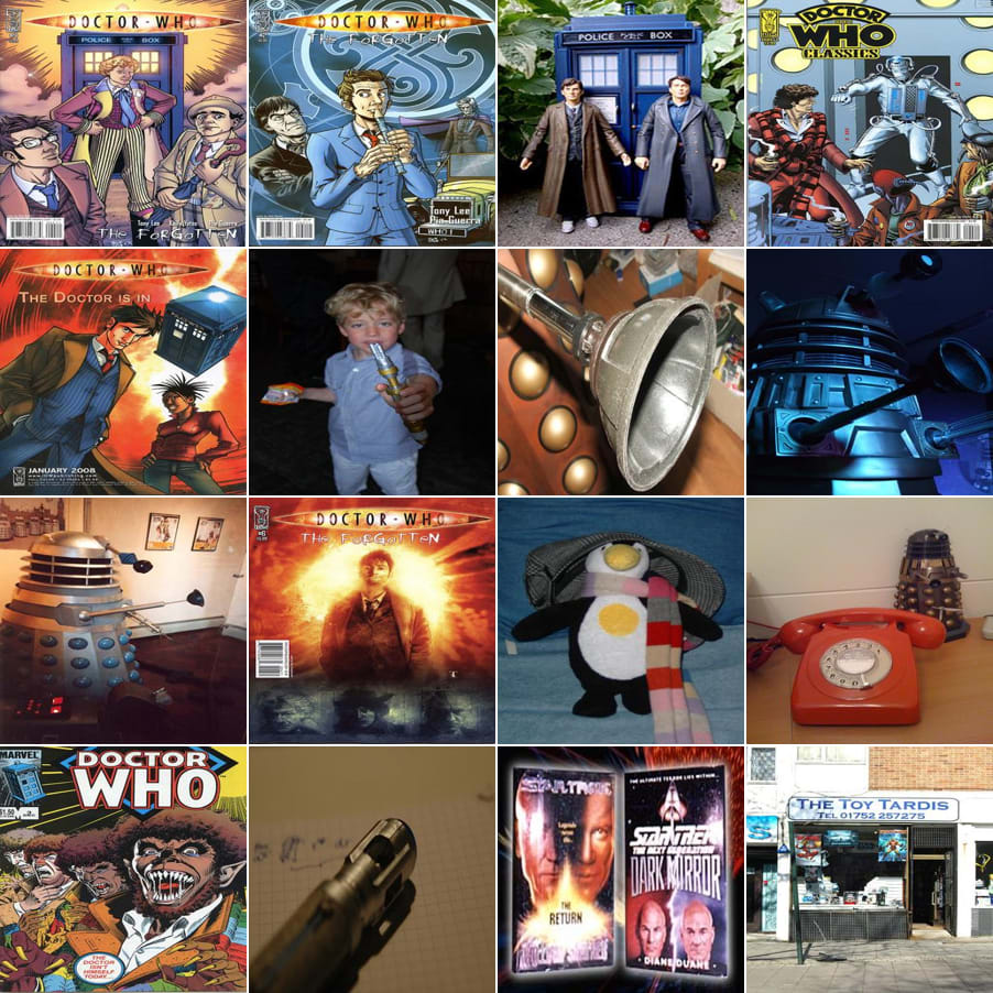
      Film/TV Features:
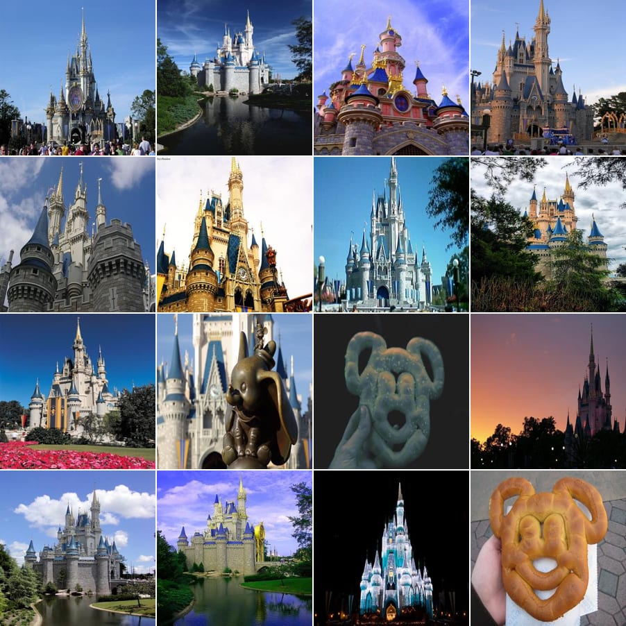
        Disney:
      Texture Features:
        Pixelation:
        Chromatic aberration:
      Miscellaneous Features:
        Mum and babies:
        Animals eating other animals:
        Repeated identical animals or people:
        Taxidermy:
        Museum exhibits:
      NSFW Features:
    How Trustworthy are Highest Activating Images?
      Tennis Feature
       Border Terrier Feature
      Mushrooms Feature
      Birds on Branches/in Foliage
  Training Performance
    Sparsity and l0
    MSE, l1 and Model Losses
  Identifying the Ultra-Low Density Cluster
  Neuron Alignment
  Future Work
None
8 comments

Executive Summary

In this post I present my results from training a Sparse Autoencoder (SAE) on a CLIP Vision Transformer (ViT) using the ImageNet-1k dataset. I have created an interactive web app, 'SAE Explorer', to allow the public to explore the visual features the SAE has learnt, found here: https://sae-explorer.streamlit.app/ (best viewed on a laptop). My results illustrate that SAEs can identify sparse and highly interpretable directions in the residual stream of vision models, enabling inference time inspections on the model's activations. To demonstrate this, I have included a 'guess the input image' game on the web app that allows users to guess the input image purely from the SAE activations of a single layer and token of the residual stream. I have also uploaded a (slightly outdated) accompanying talk of my results, primarily listing SAE features I found interesting: https://youtu.be/bY4Hw5zSXzQ.

The primary purpose of this post is to demonstrate and emphasise that SAEs are effective at identifying interpretable directions in the activation space of vision models. In this post I highlight a small number my favourite SAE features to demonstrate some of the abstract concepts the SAE has identified within the model's representations. I then analyse a small number of SAE features using feature visualisation to check the validity of the SAE interpretations. Later in the post, I provide some technical analysis of the SAE. I identify a large cluster of features analogous to the 'ultra-low frequency' cluster that Anthropic identified. In line with existing research [AF · GW], I find that this ultra-low frequency cluster represents a single feature. I then analyse the 'neuron-alignment' of SAE features by comparing the SAE encoder matrix the MLP out matrix.

This research was conducted as part of the ML Alignment and Theory Scholars program 2023/2024 winter cohort. Special thanks to Joseph Bloom for providing generous amounts of his time and support (in addition to the SAE Lens code base) as well as LEAP labs for helping to produce the feature visualisations and weekly meetings with Jessica Rumbelow. I would also like to thank Andy Arditi, Egg Syntax, Sonia Joseph and Rob Graham for useful advice and feedback in producing this post.

Since writing this post, I have found the research of  Rao et al.^[1] who have independently trained an SAE on a CLIP Vision Transformer. Their work, titled "Discover-then-Name: Task-Agnostic Concept Bottlenecks via Automated Concept Discovery", independently produce similar results under the framework of Concept Bottleneck Models (CBMs). However, in contrast to Rao et al. that uses their dictionary vectors to automatically name the extracted concepts and then construct performant task-agnostic CBMs on downstream datasets, my work analyzes properties of the trained SAEs similar to Bricken et al.. Our research was developed concurrently, in parallel and without knowledge of each other.

 

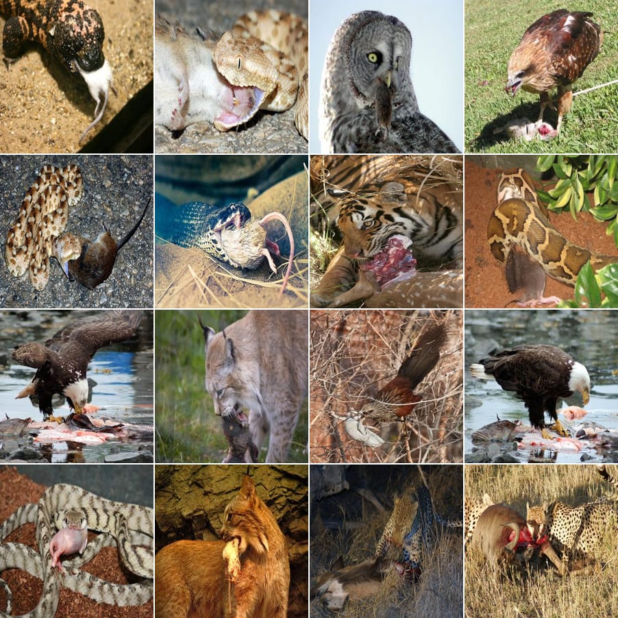
Example, animals eating other animals feature: (top 16 highest activating images)

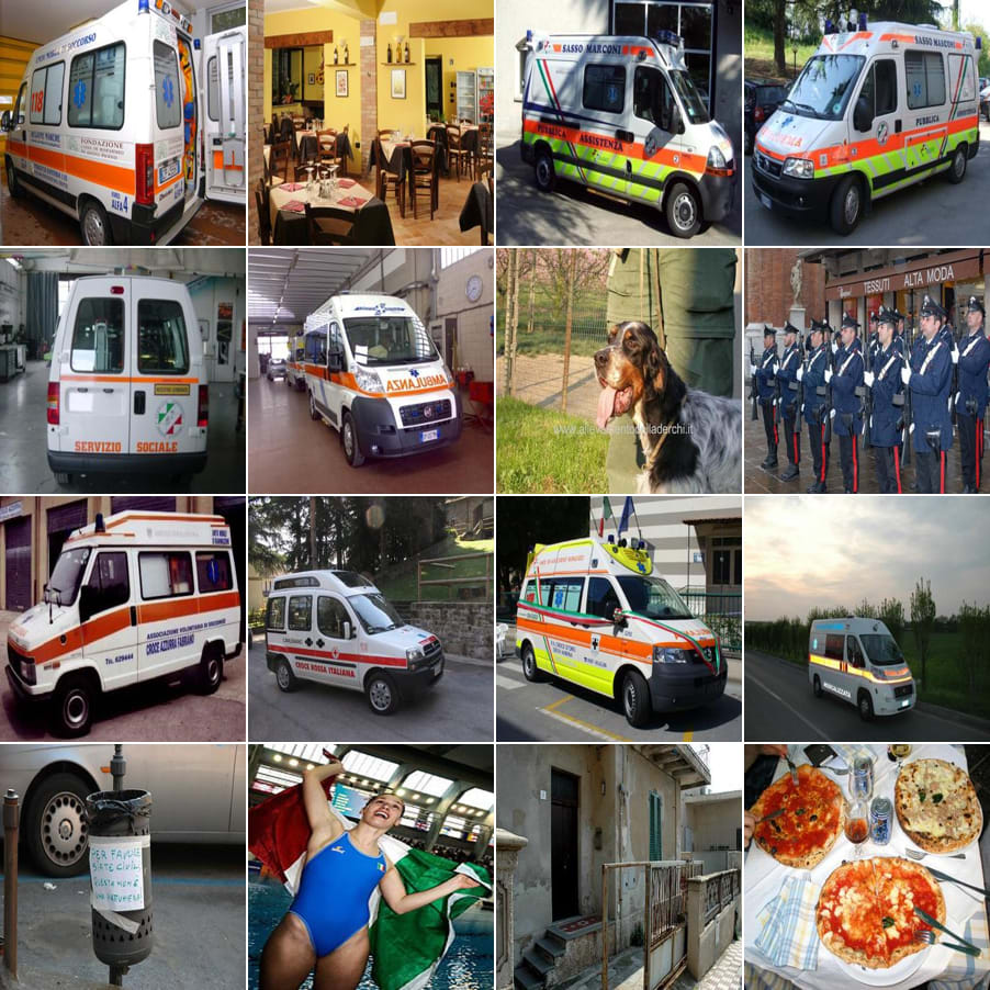
Example, Italian feature: Note that the photo of the dog has a watermark with a website ending in .it (Italy's domain name). Note also that the bottom left photo is of Italian writing. The number of ambulances present is a byproduct of using ImageNet-1k.

 

Motivation

Frontier AI systems are becoming increasingly multimodal, and capabilities may advance significantly as multimodality increases due to transfer learning between different data modalities and tasks. As a heuristic, consider how much intuition humans gain for the world through visual reasoning; even in abstract settings such as in maths and physics, concepts are often understood most intuitively through visual reasoning. Many cutting edge systems today such as DALL-E and Sora use ViTs trained on multimodal data. Almost by definition, AGI is likely to be multimodal. Despite this, very little effort has been made to apply and adapt our current mechanistic interpretability techniques to vision tasks or multimodal models. I believe it is important to check that mechanistic interpretability generalises to these systems in order to ensure they are future-proof and can be applied to safeguard against AGI.

In this post, I restrict the scope of my research to specifically investigating SAEs trained on multimodal models. The particular multimodal system I investigate is CLIP, a model trained on image-text pairs. CLIP consists of two encoders: a language model and a vision model that are trained to encode image and text in similar ways when they are from the same pair, and in dissimilar ways when they are from distinct pairs. By training in this way, information about the text is absorbed into the embeddings for the image and vice versa. CLIP is the basis of systems such as DALL-E and Stable Diffusion.

What is a Vision Transformer?

A vision transformer is a vision model with the structure of a transformer. The model works as follows:

1. An input image is resized to a standard dimensionality, in this case $[3,224,224]$ dimensions.
2. The image is broken down into a grid of $16\times 16$ image patches. Each image patch now has a dimension of $[3,14,14]$.
3. Each image patch is flattened to form a vector of size $3\times {14}^2$.
4. Each of these vectors is embedded by a shared linear map to form an embedding of a fixed dimension $d_{\text{model}}$ (in this case $d_{\text{model}}=1024$).
5. A positional embedding is added to each of the patch embeddings, before the $16\times 16$ grid of embeddings is flattened to form ${16}^2$ tokens.
6. In order to generate a single embedding vector for the whole image, an additional 'class' token is included which can attend to all the patch tokens.
7. The ${16}^2+1$ tokens are then fed into a transformer, with full attention between the image patches. The output of the class token is used as the embedding vector for the whole image.

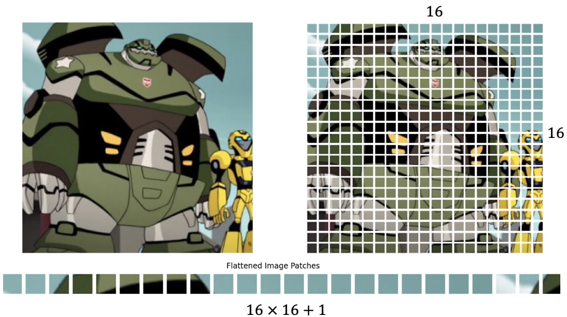
Note that by flattening each image patch before creating the embedding vectors, the ViT has to learn both the colour channels and the spatial relationships between each of the pixels. There is no locality or translation equivariance baked into the model architecture, unlike in CNNs. Despite this, ViTs are the current state of the art architecture for computer vision. For more information on ViTs I recommend the paper "An image is worth 16x16 words".

What is CLIP?

CLIP stands for Contrastive Language-Image Pre-training. CLIP consists of two models trained together: a language model encoder and a vision model encoder. The CLIP model is trained on an internet-scale dataset of (image, text) pairs. The model is trained to encode image and text in similar ways when they are from the same pair, and in dissimilar ways when they are from distinct pairs. In particular, the CLIP model is trained as follows:

1. A batch of $N$ (image, text) pairs are sampled from the dataset.
2. All images and text prompts are fed into the vision model and language model respectively to generate $N$ text encodings $T_i$ and N image encodings $I_i$.
3. The cosine similarity between each of the $N^2$ embedding pairs ($I_i$, $T_j$) is calculated to form an $N\times N$ matrix of cosine similarities.
4. A probability distribution is created for each row and column using a softmax of the cosine similarities. These probability distributions represent the probability that the image and text came from the same pair in the dataset.
5. The cross entropy loss is calculated for each row and column.
6. The total loss is taken to be the average cross entropy loss across all rows and columns.

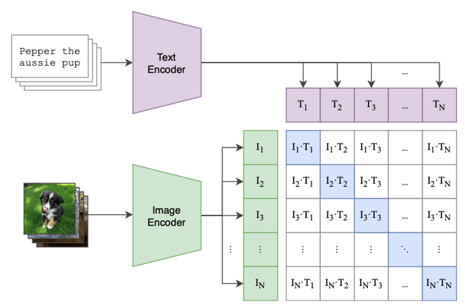
 For more information on CLIP, I recommend reading the original CLIP paper.

Training the SAE

In this post I train an SAE on the residual stream of the class token of CLIP ViT Large. The implementation details are given below: ^[2]

• Model: CLIP ViT Large.
• Location: the output of layer 22 (of 24) on the residual stream of the class token.
• Training dataset: ImageNet-1k.
• SAE expansion factor: 64.
• Total number of training images (tokens): 2 621 440 (batch size 1024).

The class token was chosen so that the SAE learns features relevant to the whole image. A later layer was chosen so that the SAE features represent more abstract concepts. I believe this is the first published research to apply SAEs to vision models or multimodal systems.

Examples of SAE Features

This section examines individual features found by the SAE. For each feature, the top 16 highest activating images are visualised in a grid. If you are only interested in the technical analysis of the SAE, I encourage you to skip to the section titled "Training Performance".

Interesting and Amusing Features

There are tonnes of interesting and amusing features, I have only included a small subset of them here. I highly encourage you to explore and find your own features in SAE Explorer (https://sae-explorer.streamlit.app/).

Era/Time Features:

These features are potentially safety relevant. Understanding how models represent time could be a first step towards understanding how they might make plans and long term goals. I have only included two such features here for brevity.

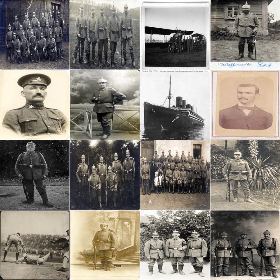
World War I Era Feature: Note the ocean liner SS Kronprinzessin Cecilie and the biplane.

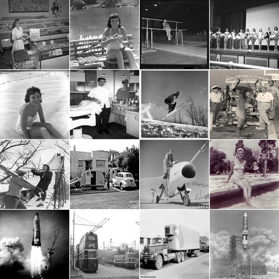
1950's Era Feature:

 

Place/Culture Features:

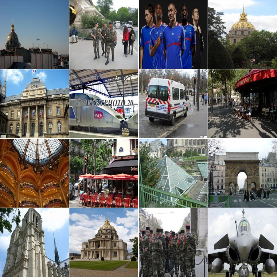
France: Check for yourself with google lens, all of these photos are of French things (including the French national football team kit, and a Dassault Rafale fighter jet).

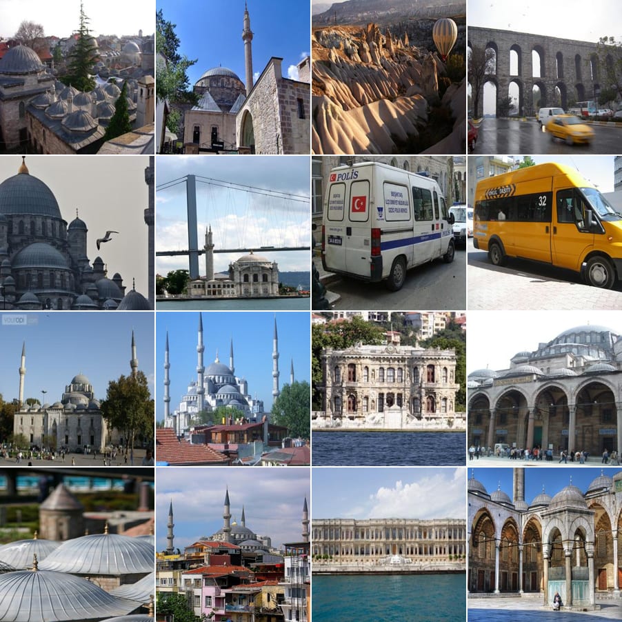
Turkey: Note the yellow Turkish school bus!

Italy: Note the photo of the dog has a watermark with a website ending in .it (Italy's domain name). Note also the bottom left is a photo of Italian writing. The number of ambulances is a byproduct of ImageNet-1k.

African Animals:

 

Film/TV Features:

Harry Potter: The number of bridges present is a byproduct of using ImageNet-1k.

Doctor Who: Notice the penguin is wearing Tom Baker's Dr Who scarf.

Disney:

 

Texture Features:

Pixelation:

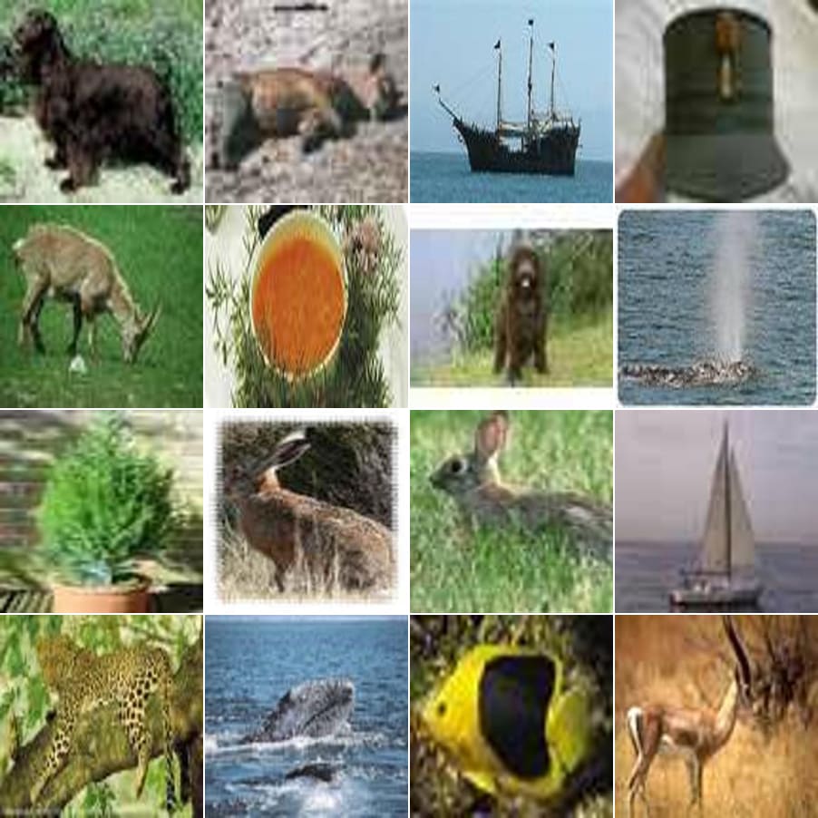
Chromatic aberration:

 

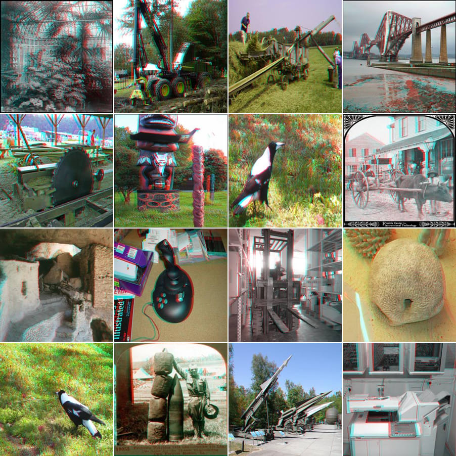
Miscellaneous Features:

Mum and babies:

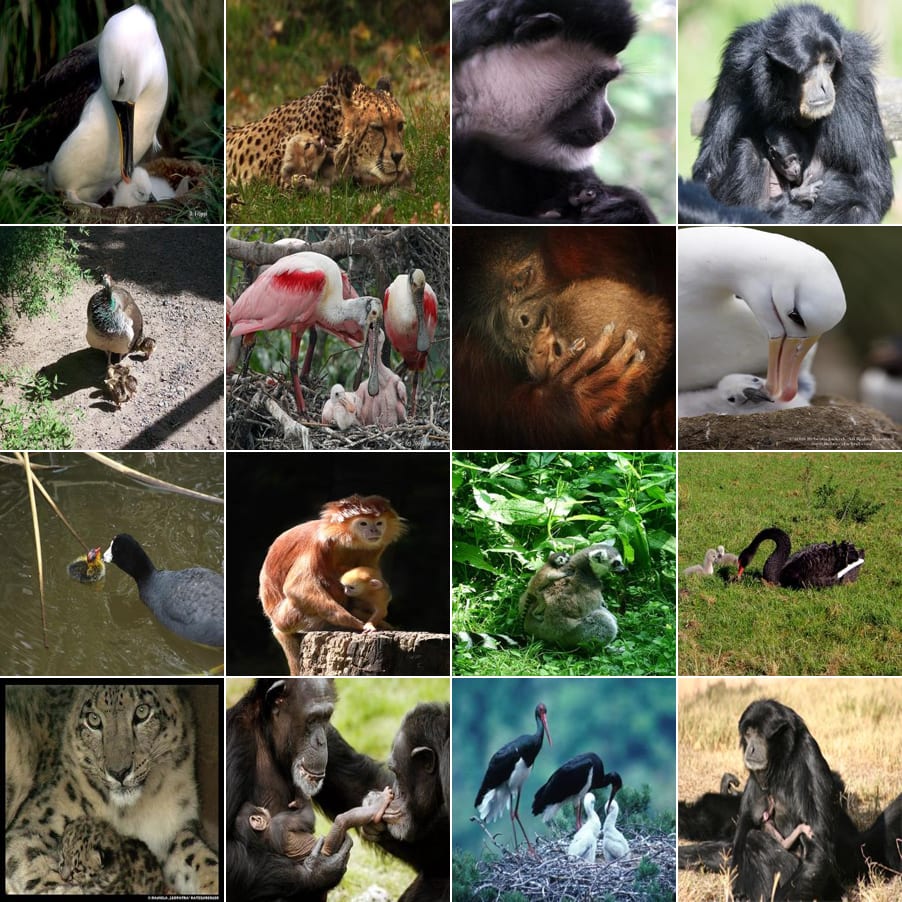
Animals eating other animals:

Repeated identical animals or people:

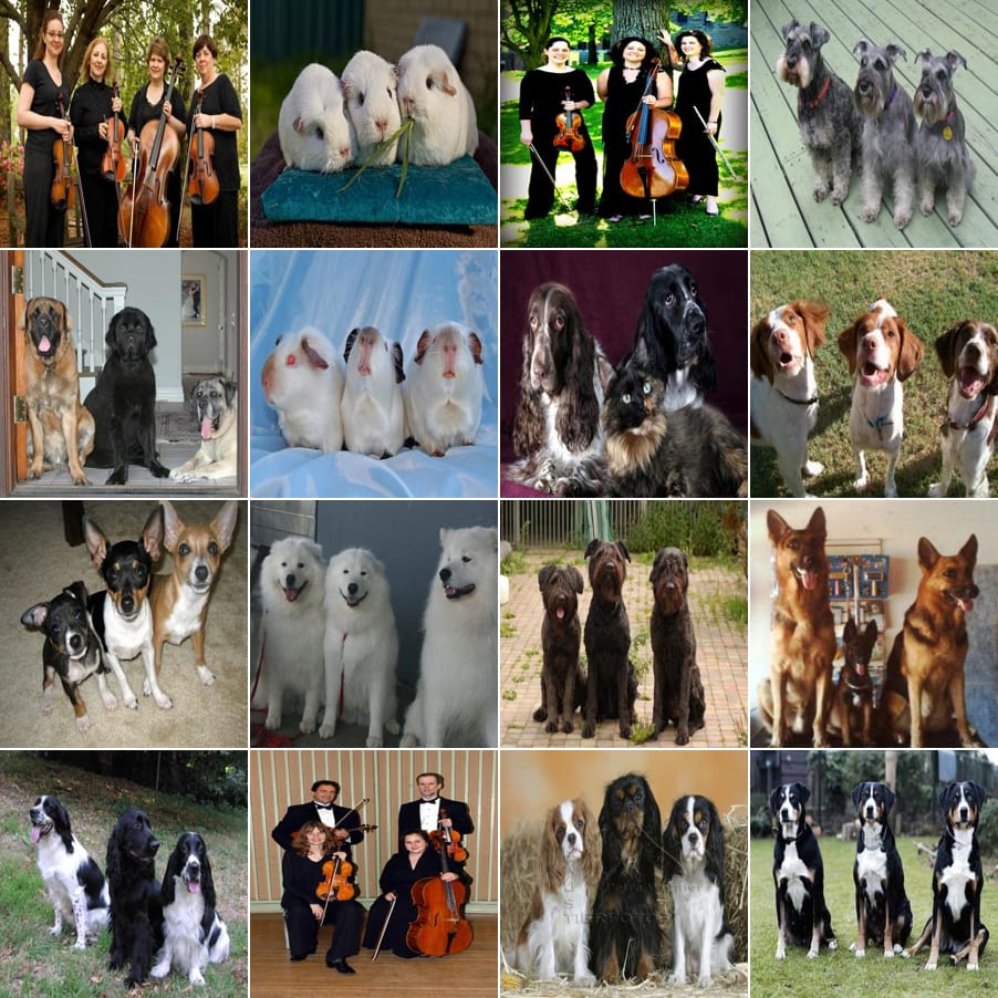
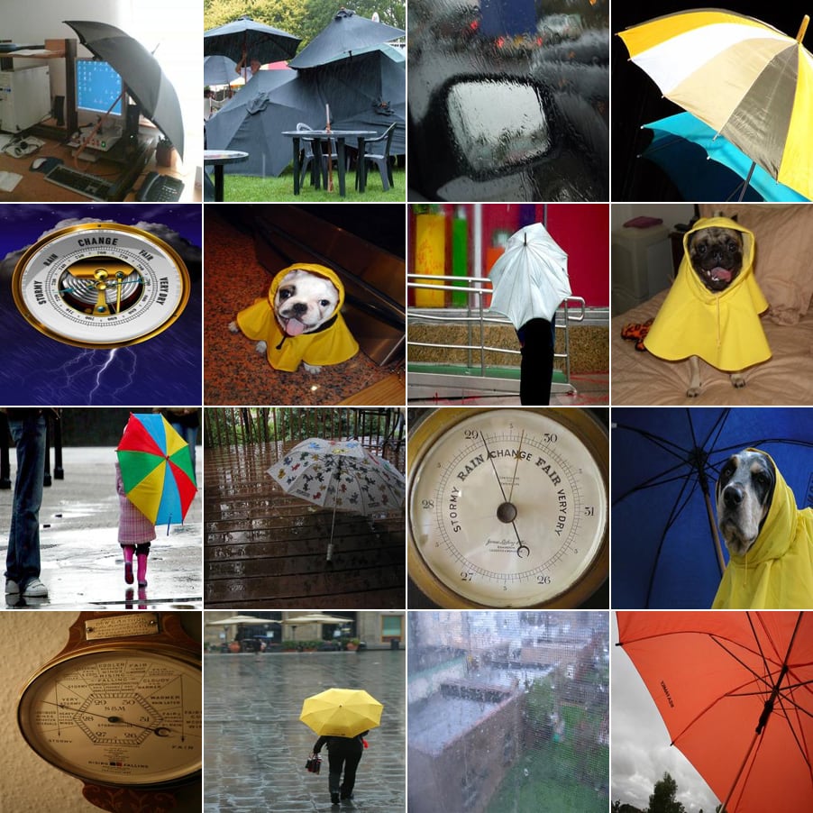
Rain: Note the rain gauges.

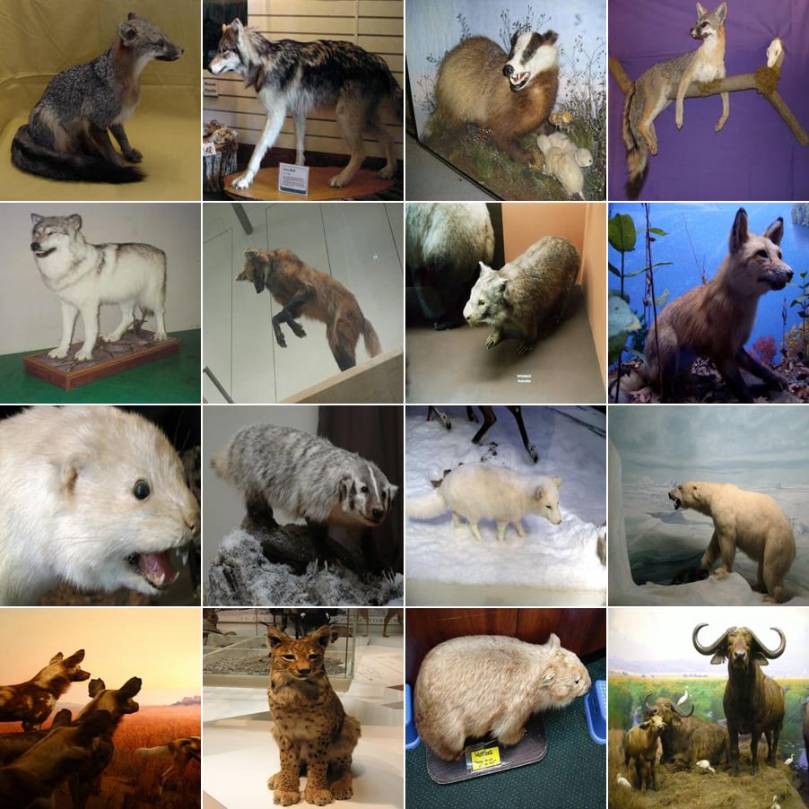
Taxidermy:

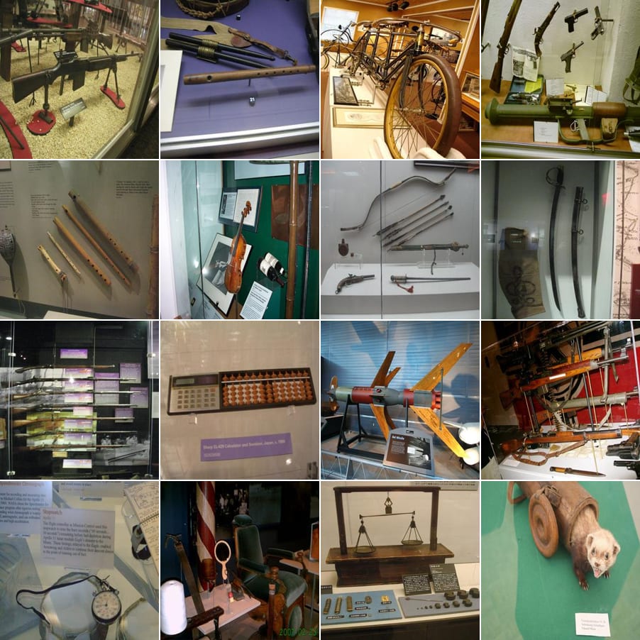
Museum exhibits:

NSFW Features:

I have not included the highest activating images of these features in this post for obvious reasons, but the curious among you can search the neuron index using the 'neuron navigator' in SAE Explorer. (NB: none of the images are graphic or disturbing.)

• Sex (including sheep and flies): index 49344.
• Violence/death: index 1417.
• Sexual fetishes: index 29775.

How Trustworthy are Highest Activating Images?

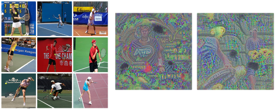
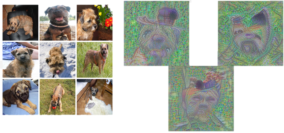
The highest activating images appear to be highly interpretable, but how can we be sure that they are faithfully representing the SAE feature? Perhaps the SAE feature is actually activating on some spurious correlation present in the highest activating images and not the feature we have identified. To answer this question, I have taken a few SAE features and generated feature visualisations from the CLIP model with the SAE. I have only included the 9 highest activating images to make space for the feature visualisations. These visualisations were created using the Leap Labs API.

Tennis Feature

Note the presence of the "ATP" in the feature visualisation - the acronym for the Association of Tennis Professionals. Note also the presence of the wrist band (common in tennis), the tennis rackets and tennis balls.

 Border Terrier Feature

Mushrooms Feature

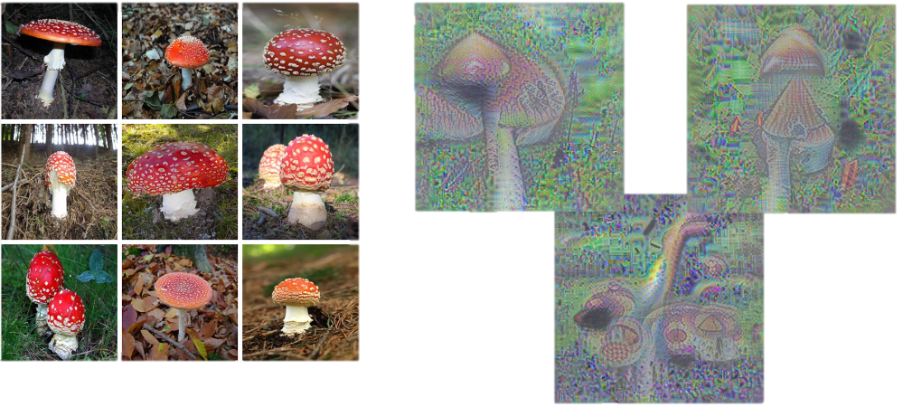
Birds on Branches/in Foliage

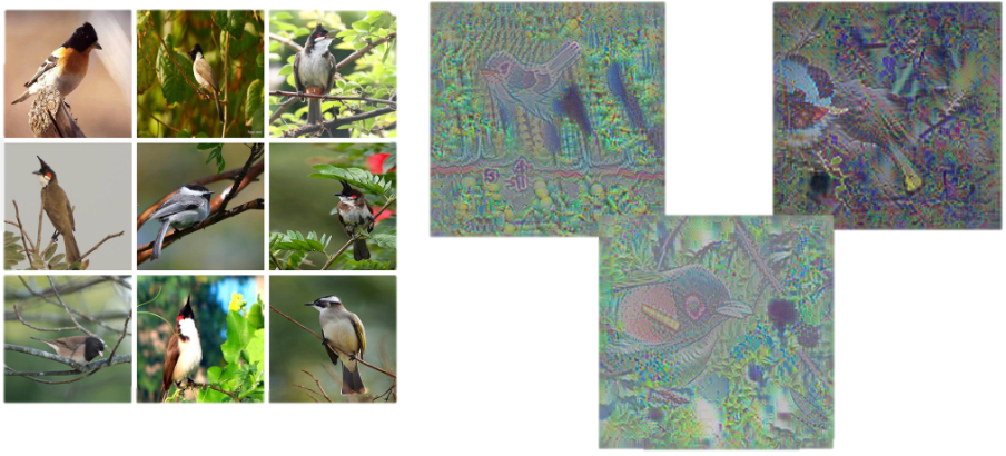
Training Performance

Sparsity and $l_0$

The sparsity of an SAE feature measures how frequently an SAE feature fires. For example, a sparsity of 0.01 means the feature fires on 1% of input images.

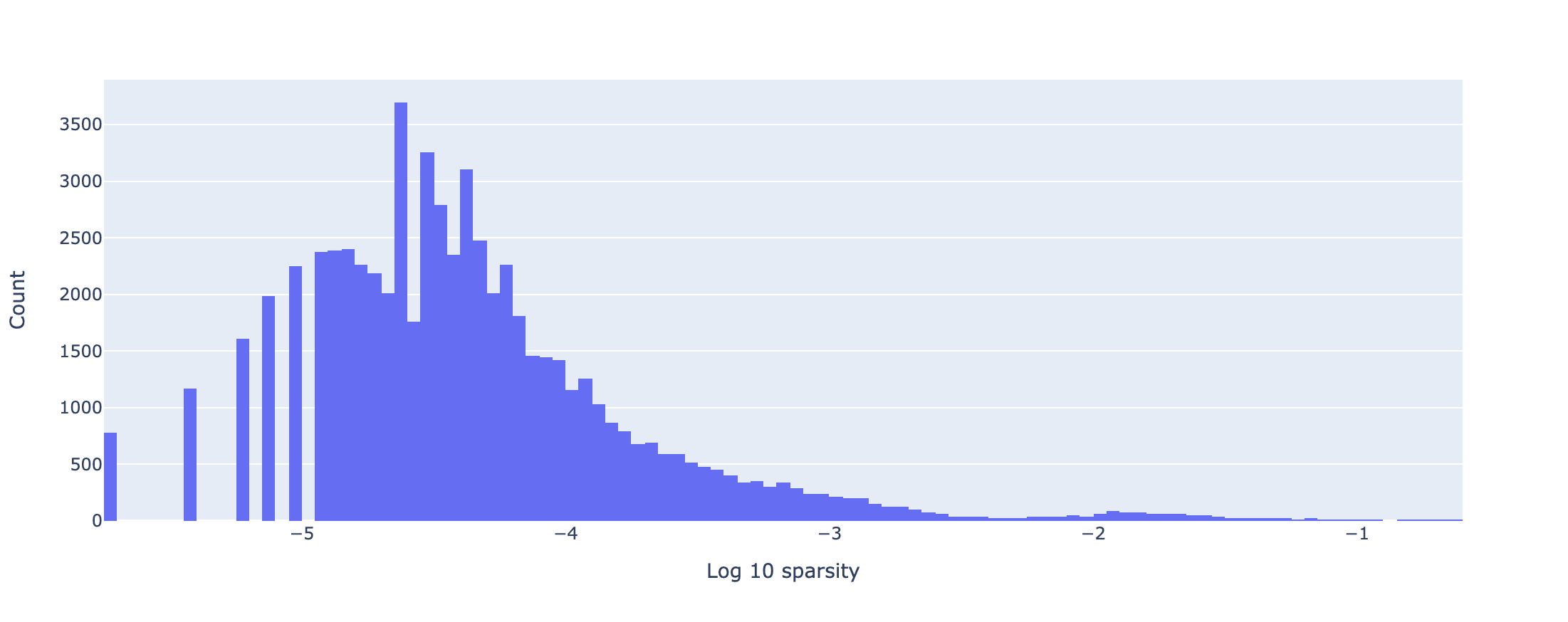
The sparsity histogram above was evaluated over 524 288 images. The histogram illustrates that none of the SAE features are dead. Additionally, the final value of $l_0$ was $l_0=26$ (the average number of SAE features that fire on an input image). These both suggest that the SAE has learnt sparse representations of the data.

MSE, $l_1$ and Model Losses

Loss type	MSE	$l_1$	Model with SAE (contrastive loss)	Original model (contrastive loss)
Value	0.0027	13.9	1.775	1.895

Note that the model with the SAE attains a lower loss than the original model. It is not clear to me why this is the case. In fact, the model with the SAE gets a lower loss than the original model within 40 000 training tokens. Further investigation is needed. Explained variance is 86%, definitely lower than I would like.

Identifying the Ultra-Low Density Cluster

The vast majority of SAE features fall into a cluster analogous to the 'ultra-low density' cluster that Anthropic identified. To show this, I have plotted the distribution of SAE features through the following three metrics:

1. ($x$-axis) ${\text{log}}_{10}\left(\text{sparsity}\right)$.
2. ($y$-axis) ${\text{log}}_{10}$(mean activation value taken across the 20 highest activating images for each feature).
3. (Colour) Label entropy: entropy of the ImageNet-1k labels across the 20 highest activating images of each feature (if 20 exist, else across the set of all images that activate the feature). The probabilities used in the entropy calculation are weighted linearly by the associated activation value.

The distribution of SAE features according to these three metrics is shown below:

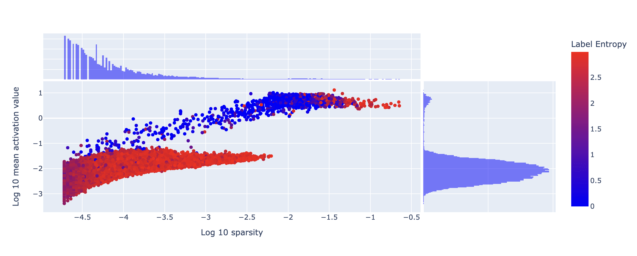
You can clearly see that the SAE features split into two clusters, most strikingly separated by the marginalised histogram for mean activation value. The lower band contains almost all of the features, and these features fire randomly on the inputs (high label entropy). The features in the upper band are also quite well separated by the label entropy, although there are some high label entropy, high density features too (discussion on these features below). The number of features in the ultra-low density cluster suggests that my expansion factor is too high. Retraining with an expansion factor of 16 (4x smaller) produces very similar results:

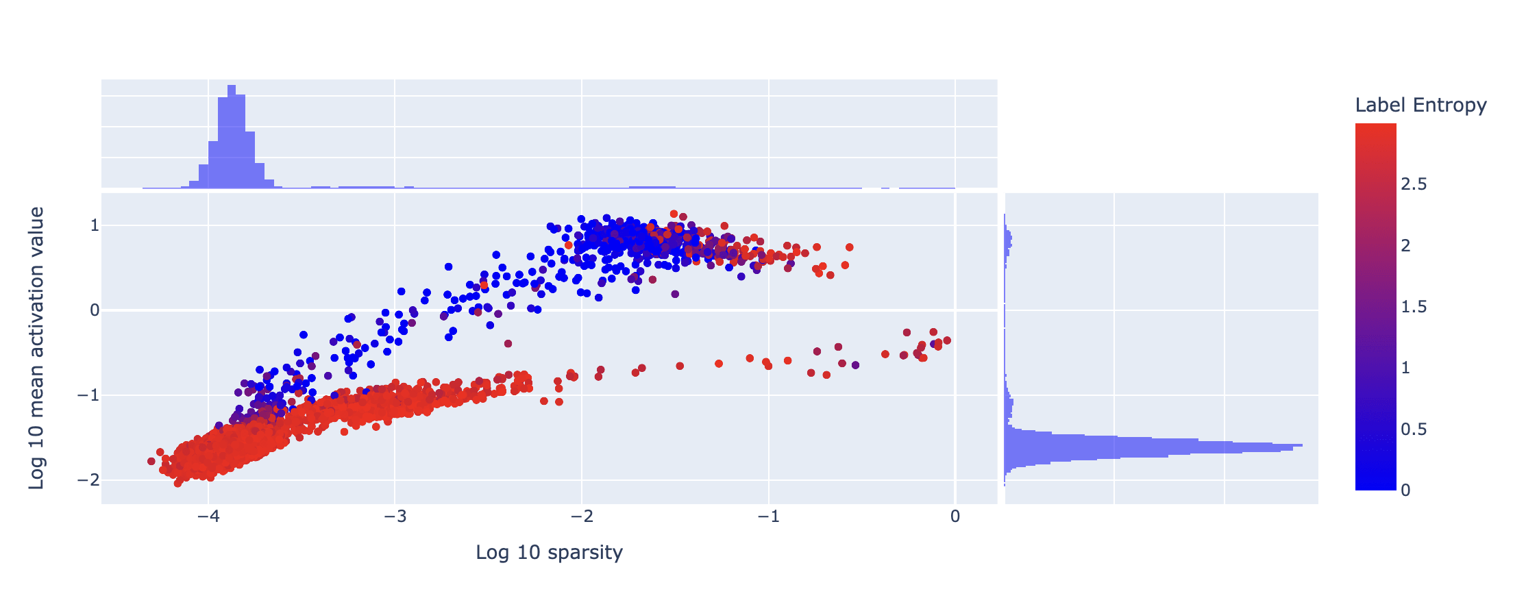
I believe the reason there are so many features in the ultra-low density cluster is a byproduct of the fact that the SAE was trained on ImageNet-1k. ImageNet-1k contains 1000 image classes with ~ 1 000 000 training images. The dataset is not very high dimensional or particularly sparse. For example, 118 of the classes are of dogs (more than 1 in 10 images), and therefore a dog feature would fire with a ${\text{log}}_{10}$ sparsity of more than -1. The CLIP model was also trained on a much larger internet scale dataset. When restricted to the ImageNet-1k dataset, I therefore suspect that a large proportion of the CLIP model's activations can be recovered with a relatively small number of features. My primary goal for the next steps of my research is to reproduce these graphs for an SAE trained on a much larger dataset such as LAION-400M, though this is currently unavailable.

Another interesting point to note is that, inline with other research [LW · GW], the ultra-low density cluster represents a single feature; the cosine similarity between feature encoder vectors in this cluster is very high. In fact for the expansion factor 16 SAE, despite having an $l_0$~26, I found an input image that caused 6458 SAE features to fire (39.42% of all SAE features).

A quick note on the label entropy distribution of SAE features in the dense cluster:

• Label entropy > 0 features in the dense cluster usually provide interesting examples of interpretable features that don't naturally align with ImageNet-1k classes. You can explore these features through SAE Explorer, but I have provided some of my favourite examples later in this post. However, some of the very high label entropy examples in the dense cluster appear completely uninterpretable. These features may be doing some dense uninterpretable linear algebra operations. It is also possible that they could be representing non-robust features present in the images and so appear uninterpretable to humans (see Adversarial Examples Are Not Bugs, They Are Features for an explanation of non-robust features). Further investigation is needed here.
• Label entropy = 0 features represent something correlated to or present in the ImageNet-1k class or a subset of the ImageNet-1k class. While label entropy = 0 features may seem boring cases where the SAE has simply learnt the class labels, they actually provide an interesting examination of the model's taxonomy within each ImageNet-1k class and may be interesting to study from the perspective of feature splitting.

Neuron Alignment

In this section, I will restrict only to non-ultra-low frequency features.

Existing vision model interpretability methods have predominantly focussed on neuron level interpretability, such as neuron feature visualisation (cf. DeepDream). This highlights the need to check whether the features the SAE has learnt are neuron aligned. In particular, in this section I analyse the similarity between the (residual stream) SAE feature encoder vectors and the MLP out vectors. Note that in the residual stream, the MLP out vectors form an over complete basis.

In the histogram below, I computed the cosine similarity between each SAE encoder vector and each MLP out vector. I then calculated the maximum cosine similarity across all the MLP vectors, for each SAE feature. I repeated this calculation for random vectors in place of the SAE encoder vectors to act as a benchmark (with the same number of random vectors as SAE features).

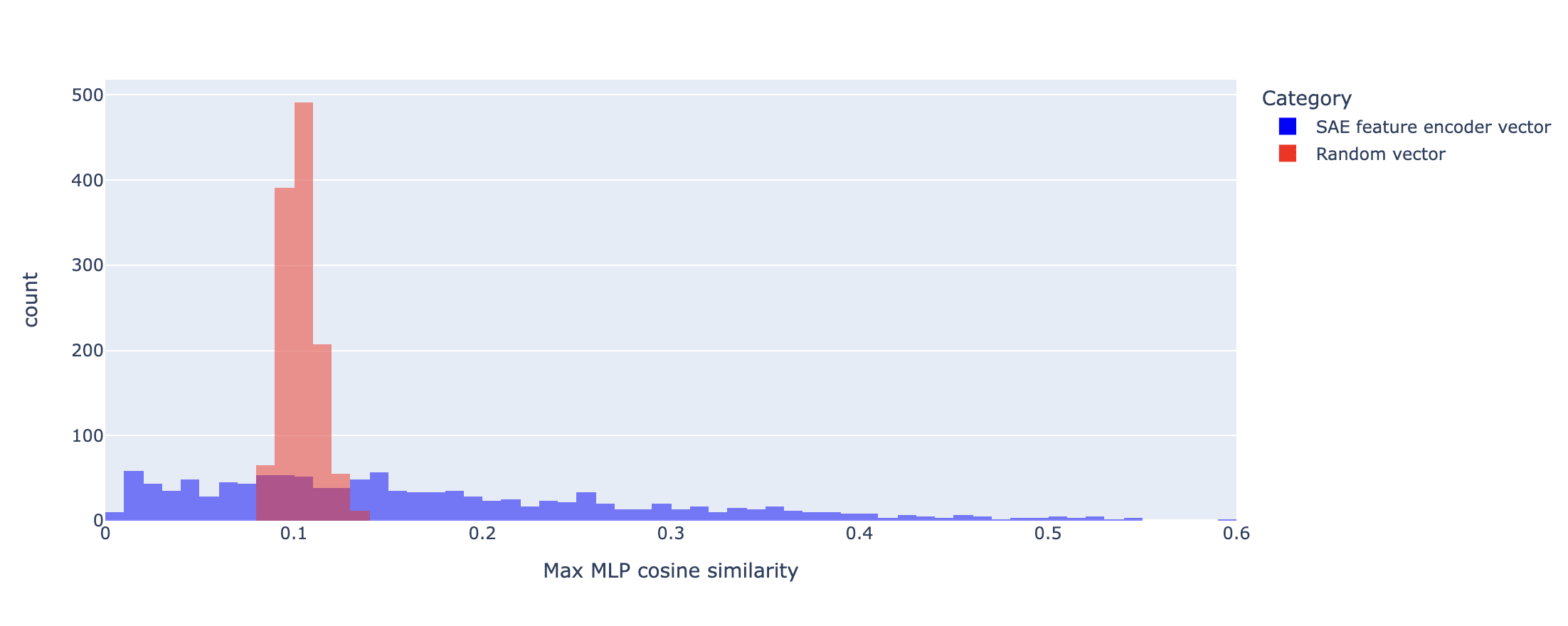
The cosine similarities for random vectors fall in the range [0.08, 0.14]. Approximately half of the SAE features fall above the random range, and half are either within or below it. A significant number of SAE features are therefore either significantly more or significantly less neuron aligned than random. By defining 'neuron aligned' to mean having a cosine similarity greater than 0.14, we can also plot the number of MLP neurons each SAE feature is aligned to:

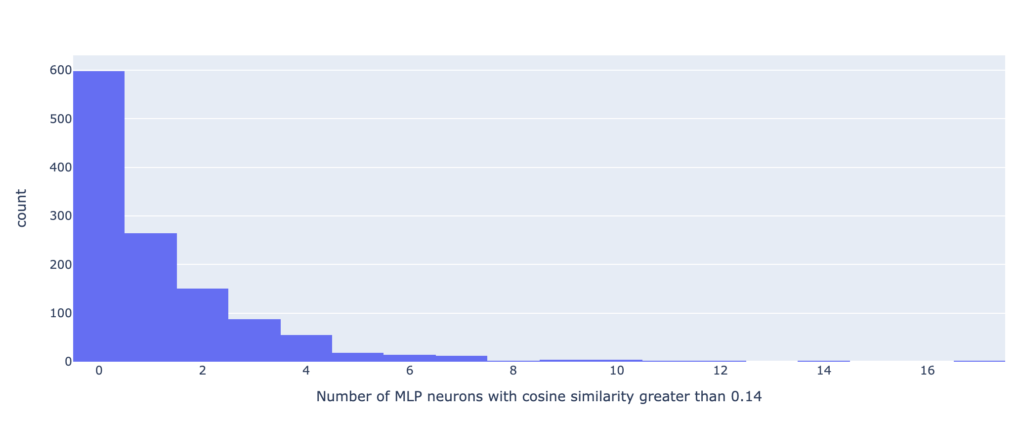
This is a very crude analysis of neuron alignment, but these results show that about a half of the features are not neuron aligned at all, and the other half are aligned mostly to a small number of MLP neurons (typically less than 5). Perhaps this is unsurprising; the SAE was trained on the residual stream just after the MLP layer, where you would expect roughly half the information present to have originated from the MLP. 

I have also generated the highest activating images for each MLP neuron and they all appear to be polysemantic, combining typically 3 or 4 unrelated features of the data (they are all much less interpretable than the SAE features). Additionally, I have analysed the neuron alignment to MLPs in earlier layers, and the results show that there is no alignment of the SAE features with any previous MLP layer (I found this surprising).

I have included cosine similarity line plots for each of the SAE neurons under the 'neuron navigator' in SAE Explorer. To get a feel for how neuron aligned the individual SAE features are, I would recommend spending five minutes in the app looking through features.

Future Work

I am intending to continue working on this research, conditional on obtaining funding. If you know of any funding bodies or individuals who would be interested in supporting this research then please leave a comment!

The most important next step is to replicate this work on a much larger internet scale dataset. I believe that many of the issues and limitations with my current research are due to training on ImageNet-1k.

After validating my results on a larger dataset, I want to train on patch tokens, across all layers. This work would be naturally integrated into the Prisma library, enabling a larger community of researchers to build on my work. This would enable me to identify 'sparse feature circuits' in the CLIP ViT model. I have a team of collaborators excited to work on this particular project. I would be particularly excited to analyse adversarial images from the perspective of sparse feature circuits.

Building a platform that displays the SAE features in an 'activation atlas' is another research direction that I find interesting, as it enables visualisations of the interactions and relationships between SAE features.

Another important direction of future work is developing better automated interpretability methods. While I have managed to get feature visualisation working, it is too hyper-parameter dependent and compute expensive to scale as an auto-interp method. I would be excited to get automated text descriptions of the SAE features working. Automated scoring of the text explanations can be achieved using ablations in conjunction with the CLIP multimodal space.

1. ^{^}

   Rao, S., Mahajan, S., Böhle, M., & Schiele, B. (2024). Discover-then-Name: Task-Agnostic Concept Bottlenecks via Automated Concept Discovery. In Proceedings of the European Conference on Computer Vision (ECCV).

2. ^{^}

   The SAE was trained with ghost grads and used the geometric median to initialise the decoder bias. The following hyper-parameters were used. learning rate: 0.0004 (with a linear warm up). l_1 coefficient: 0.00008.

8 comments

Comments sorted by top scores.