Grokking revisited: reverse engineering grokking modulo addition in LSTM

post by Nikita Khomich (nikitoskh), Danik (daniil-yurshewich) · 2024-12-16T18:48:43.533Z · LW · GW · 0 comments

Contents

  Introduction
  Model architecture, experiment settings and naming conventions 
    Exact formulas for what LSTM does  
      Model Parameters and Dimensions
      Input Encoding
      Step-by-Step for Two Steps
      Final Two Linear Layers
      Final Output
  Reverse engineering the model
    Reducing the problem to simplified model
    Reverse engineering simplified model 
    The algorithm itself
      Three important points
    Summary 
None
No comments

By  Daniil Yurshevich, Nikita Khomich

 

TLDR: we train LSTM model on algorithmic task of modulo addition and observe grokking. We fully reverse engeneer the algorithm learned and propose a way simpler equivalent version of the model that groks as well. 

Reproducibility statement: all the code is available at the repo.

Introduction

This post is related to Neel Nanda's [LW · GW] post and a detailed description of what grokking is can be found there. The short summary is that grokking is the phenomenon when model when being trained on an algorithmic task of relatively small size initially memorizes the trining set and then suddenly generalizes to the data it hasn't seen before. In our work we train a version of LSTM on modulo addition and observe grokking. 

Model architecture, experiment settings and naming conventions 

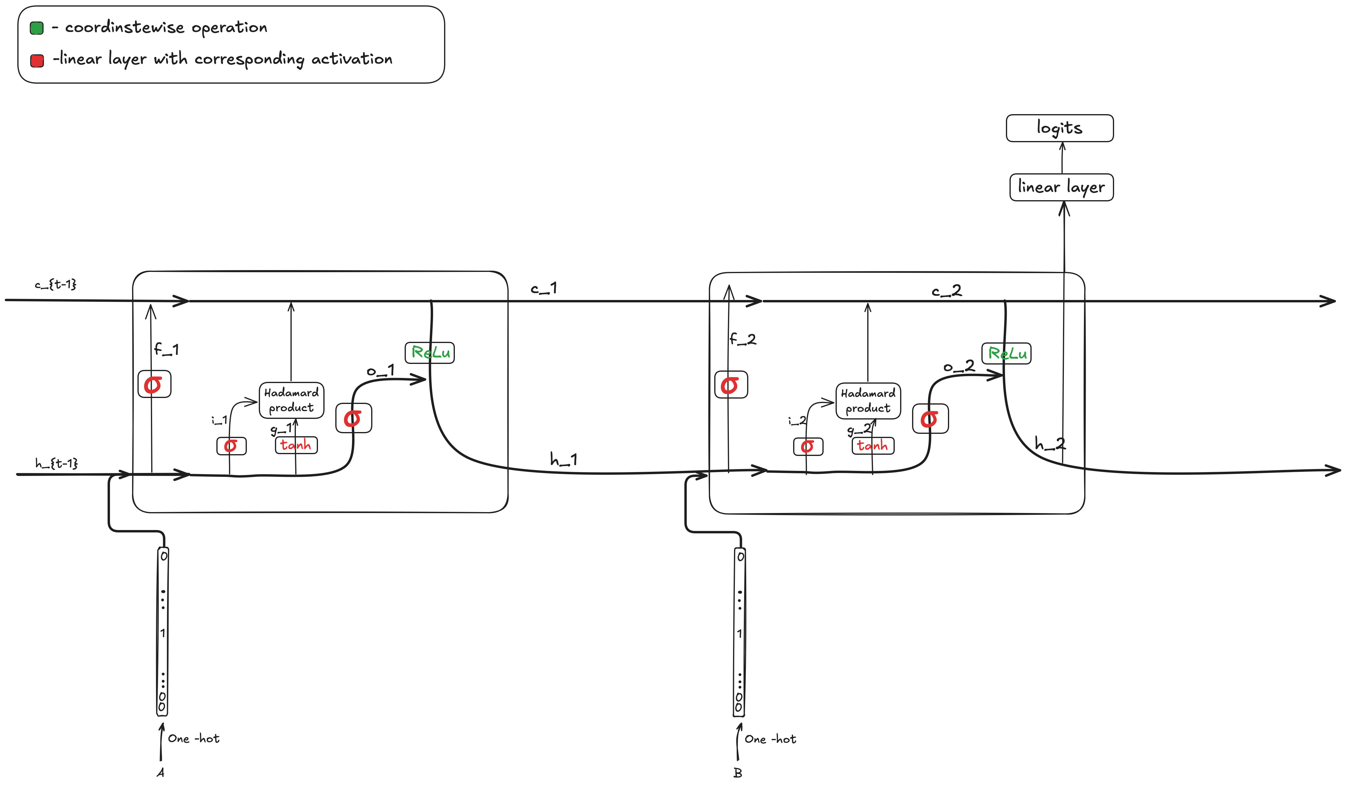
We train a version of LSTM with ReLU activation instead of $tanh$ for getting hidden state from cell state $c_t$. We use a linear layer without bias to get logits from $h_2$. We use a slight trick which is using two linear layers without activation inbetween instad of one which makes grokking easier. We also use hidden dimension of $N=p$ and one-hot encoded embeddings. The exact model arcitecture as well as naming is (very similar to Chris Olah's amazing post) 

We use similar parameters to Neel's paper meaning extremely large weight decay and particular set of betas for Adam found with grid search. We train the model on a 30% of all pairs $(a,b)mod113$ and observe grokking: 

 

 

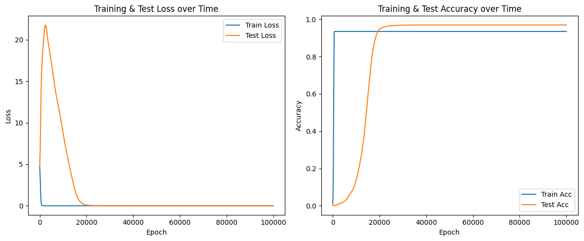
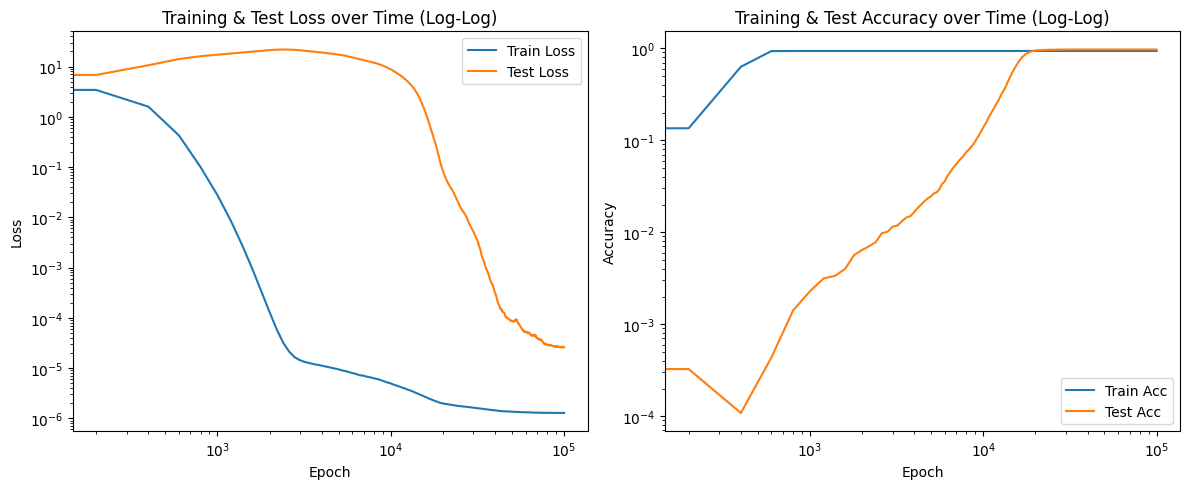
This is a typical and well studied behaviour for transformer, however we are not aware of any examples of reverse enginnered problem with observed grokking during training. 

Exact formulas for what LSTM does  

This section is only relevant to the methodology we used to reverse engineer the model, not understanding algorithm itself as well as clarifying all the architectural details used, so feel free to skip this section.

Below are the formulas describing all intermediate activations and operations performed by the given model architecture. The model predicts $a+b\mathrm{mod}113$ from inputs$a,b\in \{0,\dots ,112\}.$

Model Parameters and Dimensions

N = 113 (the modulo and also number of classes)

$\text{vocab\_size}=N$

$\text{hidden\_size}=113$

The input is a pair $(a,b)$ with $a,b\in \{0,\dots ,N-1\}.$

Input Encoding

We have an input sequence of length 2:

$x\_seq\in R^{\text{batch}\times 2},x\_seq[i,0]=a,x\_seq[i,1]=b.$

We one-hot encode each integer:

$x_{onehot}[i,0,:]=\text{one\_hot}\left(a\right),x_{onehot}[i,1,:]=\text{one\_hot}\left(b\right).$

Thus:

$x_{onehot}\in R^{\text{batch}\times 2\times \text{vocab\_size}}.$
LSTM-like Cell Parameters

We have a single-layer LSTM-like cell with parameters:

$W_{ih}\in R^{4\cdot \text{hidden\_size}\times \text{vocab\_size}},b_{ih}\in R^{4\cdot \text{hidden\_size}}$

$W_{hh}\in R^{4\cdot \text{hidden\_size}\times \text{hidden\_size}},b_{hh}\in R^{4\cdot \text{hidden\_size}}$

These define the input, forget, cell (g), and output gates at each timestep.

$h_0=0\in R^{\text{hidden\_size}},c_0=0\in R^{\text{hidden\_size}}.$

Recurrent Step $(t=0,1)$

$For(t\in \{0,1\}:x_t=x\_onehot[:,t,:]\in R^{\text{batch}\times \text{vocab\_size}}$

Compute gates:

$\text{gates}=W_{ih}{x}_t^T+b_{ih}+W_{hh}{h}^T+b_{hh}$

which results in a $\text{batch}\times (4\cdot \text{hidden\_size})$ vector.

Slice into four parts:

$i_t=\sigma \left(\text{gates}\right[:,0:\text{hidden\_size}\left]\right)$

$f_t=\sigma \left(\text{gates}\right[:,\text{hidden\_size}:2\cdot \text{hidden\_size}\left]\right)$

$g_t=\tanh \left(\text{gates}\right[:,2\cdot \text{hidden\_size}:3\cdot \text{hidden\_size}\left]\right)$

$o_t=\sigma \left(\text{gates}\right[:,3\cdot \text{hidden\_size}:4\cdot \text{hidden\_size}\left]\right)$

Update cell and hidden states:

$c_t=f_t\odot c_{t-1}+i_t\odot g_t$

However, instead of the standard LSTM update $h_t=o_t\odot \tanh \left(c_t\right)$ , the model uses:

$h_t=\text{ReLU}\left(c_t\right)$

Step-by-Step for Two Steps

At$t=0:$

$c_1=f_0{c}_0+i_0{g}_0=i_0{g}_0\text{since}{c}_0=0$

$h_1=\text{ReLU}\left(c_1\right)$

At $t=1$:

$c_2=f_1{c}_1+i_1{g}_1$

$h_2=\text{ReLU}\left(c_2\right)$

After these two steps, $h_2$ is the final hidden state for the sequence.

Final Two Linear Layers

The final output is computed by two linear layers without bias or nonlinearities:

$\text{intermediate}=\text{fc1}\left(h_2\right)=W_1{h}_2$

$\text{logits}=\text{fc2}\left(\text{intermediate}\right)=W_2\left(\text{intermediate}\right)$

Where:

$W_1\in R^{\text{hidden\_size}\times \text{hidden\_size}},W_2\in R^{\text{vocab\_size}\times \text{hidden\_size}}$

No bias and no additional activations are applied here.

Final Output

$\text{logits}\in R^{\text{batch}\times \text{vocab\_size}}$

The model’s output is the $\text{logits}$ vector for each sample, which can be turned into a probability distribution via softmax.

Reverse engineering the model

Reducing the problem to simplified model

Turns out model prefers to learn way simpler structure and not use the full capability of LSTM. We find the following: 

• $f_t$ is constant and the accuracy on the test set  does not change if we replace f_t with constant vector equal to the average over the train set.
• $i_t$ can be replaced by tensor of ones. that does not change the accuracy. 
• $o_t$  can be replaced by tensor of ones. that does not change the accuracy. 
• $tanh$ after the linear layer when computing $g_t$  from can be removed and does not affect the accuracy ($tanh\left(x\right)$ is close to x for small values).

• $ReLU$ applied in the first cell to $c_1$ when computing $h_1$ can be removed with no accuracy drop.

   

   

   

Given the above the model architecture simplifies to: 

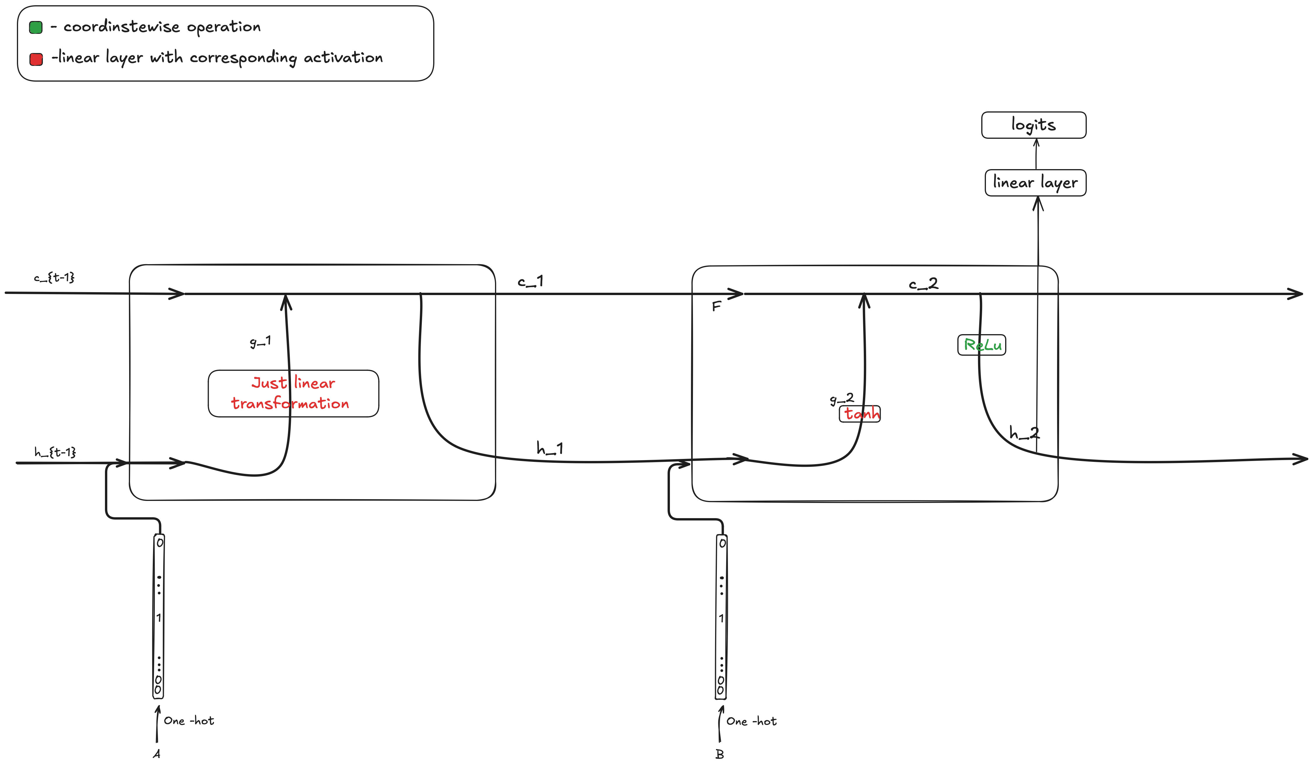
This allows us to simplify the formula for $C_2$ significantly: 

$C_2=F\left(W_g^{ih}E\right(a)+b_g)+W_g^{hh}ReLU\left(W_g^{ih}E\right(a)+b_g)+b_g+W_g^{ih}E\left(b\right)$

Which can be written as 

$C_2=\left(F\right(W_g^{ih}E\left(a\right)+b_g)+W_g^{hh}ReLU(W_g^{ih}E\left(a\right)+b_g)+b_g)+\left(W_g^{ih}E\right(b\left)\right)$

Where $E\left(a\right)$  and $E\left(b\right)$ are one hot encodes numbers and F is a constant $f_t$.

Now we can see that the two summands are just functions of $a$ and $b$ and given $W_g^{hh}$ those can be considered to have capacity to learn almost any representations independent of each other. Regardless of the interpretation the expression is just a sum of two vectors of dimension $113$ one of which is a function of $a$ only and second is a function of $b$  only. This suggest the idea of considering them just like a lookup table of embeddings for $a$ and $b$, hence we do it reducing the problem for the following: 
 

 

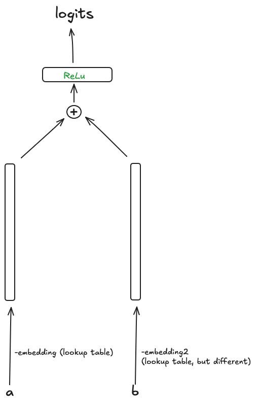
We have two different lookup tables (different or at least they have seemingly no reason to be the same based on our formula). We then take two embeddigs apply ReLU and multiply by some matrix to get logits. 

The first lookup table maps 

$a\to \left(F\right(W_g^{ih}E\left(a\right)+b_g)+W_g^{hh}ReLU(W_g^{ih}E\left(a\right)+b_g)+b_g)$

Second is 

$b\to W_g^{ih}E\left(b\right)$

We extract all the weights from the original model only in a way described above to get a simplified model. The accuracy measured for the simplified model is only 5 percent lower than the original model hence we only need to interpret the simplified model.

 

An interesting observation is that if we were to train just simplified model with the same trick by breaking down the linear layer after ReLU into the product of two matrices without activation: $W=W_1{W}_2$ the simplified model would also grok leaning the same algorithm but it would not grok with just one matrix. The idea why this is the case will become more clear after understanding the algorithm. 

 

Reverse engineering simplified model 

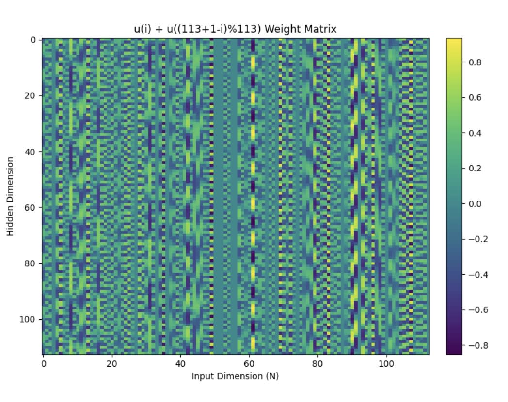
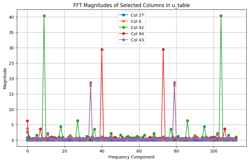
First thing we notice is that both embedding tables are highly periodic but not only that, they are almost identical and the accuracy does not drop.

Periodicity shows up in FFT plots as well: 

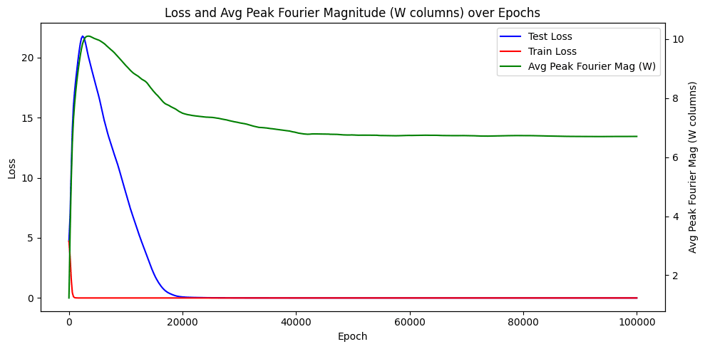
Interestingly, the average peak fourier magnitude over the training run looks like: 

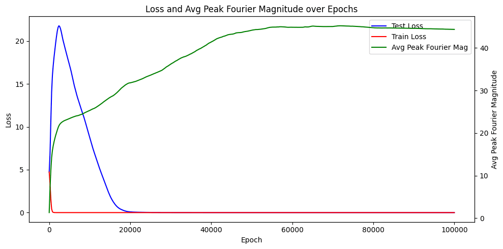
Which is explained by spasticity of frequencies used in W. Indeed, the embedding tables become periodic during the first few epochs and during the rest of the training the models learns to diversify firing activations for logits amongst many frequencies: 

The algorithm itself

We first have to provide some facts about the embeddings we observed.

Three important points

•  Each column of u is a periodic function with a non-zero magnitude only at 0 and $(-f,f)$  frequancy for some $x.$ (reminder: embeddings themselves are rows of u).
• For each integer $s$ modulo 113 the matrix with $i$ -th row equal to $u\left[i\right]+u[s-i]$ - just the sums of embeddings corresponding to pairs of integers with a particular sum, staked vertically, has highly periodic columns. Not only that, but the frequency of the $j$-th column of matrix $W$ is the same as the frequency of matrix constructed above for $s=j.$

• Columns of $W$ have just one dominant frequency, so highly periodic. 

  Below are some visualisation of the above points.

   

  

  

  

  

So the idea is if the columns present seem to be just a one magnitude wave, lets just write dows the formula for logits in assuming one dominant frequency and the expression for logits is not that complicated at this point. 

Lets look at the logits: 

Assuming observed periodicity and ignoring ReLU(which is reasonable to do because we care about periodic fucntions and as we care about scalar products of those and as matrices W and U have similar frequencies a natural thing to do is examing what is happening without ReLU)

Observe that constant term for columns of $W$ is $0$ and they have same frequancy as corresponding columns of $u$. Now $s^{\prime }$ -th logit is

 ${\sum }_{k}W\left[s^{\prime }\right]\left[k\right](u\left[j\right]\left[k\right]+u[s-j]\left[k\right])=$

${\sum }_k(((x_k+y_{k}i)e^{2\pi is\frac{f_k}{113}}+(x_k-y_{k}i)e^{-2\pi is\frac{f_k}{113}})(2c_0+(a+bi)(e^{-2\pi is\frac{f_k}{113}}+1)e^{2\pi is\frac{f_{k}j}{113}}+(a-bi)(e^{2\pi is\frac{f_k}{113}}+1)e^{-2\pi is\frac{f_{k}j}{113}}))$

So after some algebra, we find that $s^{\prime }$-th logit is  $c_{s^{\prime }}^{\prime }+e^{2\pi ij\frac{f_k}{113}}\left(\right({\sum }_k{c}_k^{\prime }{e}^{2\pi i\frac{f_k}{113}(s^{\prime }-s)})+{\sum }_k{c}_k^{\prime \prime }{e}^{2\pi i\frac{f_k}{113}(s^{\prime }+s)})+c_{s^{\prime }}^{\prime \prime })$

 

Now $c_{k^{\prime }}$ and $c_{k^{\prime \prime }}$ are of similar magnitude (being $a_k{x}_k+b_k{y}_k$ and $a_k{x}_k+b_k{y}_k$ respectively) hence the two sums above sum up to a constant  when $s^{\prime }$ is not equal to $s$ or$-s$ and $f_k$ spans all integers from 0 to 112 and the sum is just slightly noisy sum of roots of unity. The way model distinguishes them is by finding the correct $c_{s^{\prime }}$ which the model has to learn for each particular sum.

 

Summary 

We have observed that grokking and learned that the algorithm learned is still to a large extend empirical: the model has to learn those 113 values of $c^{\prime }$ separately and when it does the model groks.  So the model chose to learn 113 parameters rather then ${113}^2$ and use the fact that (weighted) sum of roots of unity is comparatively small to the sum of 1's. This is confirmed by the fact that if we reshuffle the training data not containing particular sum, the model is more likely to get it wrong. 

0 comments

Comments sorted by top scores.