A Mechanistic Interpretability Analysis of Grokking
post by Neel Nanda (neel-nanda-1), Tom Lieberum (Frederik) · 2022-08-15T02:41:36.245Z · LW · GW · 48 commentsThis is a link post for https://colab.research.google.com/drive/1F6_1_cWXE5M7WocUcpQWp3v8z4b1jL20
Contents
  Introduction
  Key Claims
  Phase Changes
    Key Takeaways
    What Is A Phase Change?
    Empirical Observations
      Grokking = Phase Changes + Regularisation + Limited Data
    Explaining Grokking
      Speculation: Phase Changes Are Inherent to Composition
      An Intuitive Explanation of Grokking
    Speculation: Phase Changes are Everywhere
    Summary
  Modular Addition
    Key Takeaways
    Model Details
    Overview of the Inferred Algorithm
    Background on Discrete Fourier Transforms
    Reverse Engineering the Algorithm
      Calculating waves cos(wx),sin(wx),cos(wy),sin(wy)
      Calculating 2D products of waves cos(wx)cos(wy),cos(wx)sin(wy),sin(wx)cos(wy),sin(wx)sin(wy)
      Calculating cos(w(x+y)),sin(w(x+y)) and calculating logits
    Evolution of Circuits During Training
  Discussion
    Alignment Relevance
    Limitations
    Future Directions
  Meta
    Notable Observations
    Acknowledgements
    Author Contributions
    Feedback
    Citation Info
None
48 comments
A significantly updated version of this work is now on Arxiv and was published as a spotlight paper at ICLR 2023
aka, how the best way to do modular addition is with Discrete Fourier Transforms and trig identities
If you don't want to commit to a long post, check out the Tweet thread summary
Introduction
Grokking is a recent phenomena discovered by OpenAI researchers, that in my opinion is one of the most fascinating mysteries in deep learning. That models trained on small algorithmic tasks like modular addition will initially memorise the training data, but after a long time will suddenly learn to generalise to unseen data.
This is a write-up of an independent research project I did into understanding grokking through the lens of mechanistic interpretability. My most important claim is that grokking has a deep relationship to phase changes. Phase changes, ie a sudden change in the model's performance for some capability during training, are a general phenomena that occur when training models, that have also been observed in large models trained on non-toy tasks. For example, the sudden change in a transformer's capacity to do in-context learning when it forms induction heads. In this work examine several toy settings where a model trained to solve them exhibits a phase change in test loss, regardless of how much data it is trained on. I show that if a model is trained on these limited data with high regularisation, then that the model shows grokking.
One of the core claims of mechanistic interpretability is that neural networks can be understood, that rather than being mysterious black boxes they learn interpretable algorithms which can be reverse engineered and comprehended. This work serves as a proof of concept of that, and that reverse engineering models is key to understanding them. I fully reverse engineer the inferred algorithm from a transformer that has grokked how to do modular addition [AF · GW] (which somehow involves Discrete Fourier Transforms and trig identities?!), and use this as a concrete example to analyse what happens during training [AF · GW] to understand what happened during grokking. I close with discussion [AF(p) · GW(p)] and thoughts on the alignment relevance [AF · GW] of these results.
This is accompanied by a paper in the form of a Colab notebook containing the code for this project, a lot of interactive graphics, and much more in-depth discussion and technical details. In this write-up I try to give a high-level conceptual overview of the claims and the most compelling results and evidence, I refer you to the notebook if you want the full technical details.
This write-up ends with a list of ideas for future directions of this research [AF · GW]. I think this is a particularly exciting problem to start with if you want to get into mechanistic interpretability since it's concrete, only involves tiny models, and is easy to do in a Colab notebook. If you might want to work on some of these, please reach out! In particular, I'm looking to hire an intern/research assistant, and if you're excited about these future directions you might be a good fit.
Key Claims
- Grokking is really about phase changes [AF · GW]: To exhibit grokking, we train a model on a problem that exhibits phase changes even when given infinite training data, and train it with regularisation and limited data. If we choose the amount of data such that the regularisation only marginally favours the generalising solution over the memorised solution, we see grokking.
- Intuition: Regularisation makes the model ultimately prefer the generalising solution to the memorised solution, but the phase change indicates that the generalising solution is "hard to reach" in some sense. The memorised solution is "easier to reach", and so is reached first. But due to the regularisation, the model still prefers the generalising solution to the memorised solution, and thus gets to the generalising solution eventually - the grokking result just shows that reaching the memorised solution first does not change this, and that there is a path in model space interpolating between the memorising and generalising solution.
- The algorithm learned to do modular addition can be fully reverse engineered [AF · GW]. The algorithm is roughly:
- Map inputs with a Discrete Fourier Transform, for some frequency
- Multiply and rearrange to get and
- By choosing a frequency we get period dividing n, so this is a function of
- Map to the output logits with - this has the highest logit at , so softmax gives the right answer.
- To emphasise, this algorithm was purely learned by gradient descent! I did not predict or understand this algorithm in advance and did nothing to encourage the model to learn this way of doing modular addition. I only discovered it by reverse engineering the weights.
- The generalising circuits used to do modular addition can be seen to smoothly evolve over the course of training [AF · GW], as the model interpolates between purely memorising and purely generalising
- In particular, the circuits smoothly develop well before grokking, disproving the 'grokking is a random walk in model-space' hypothesis.
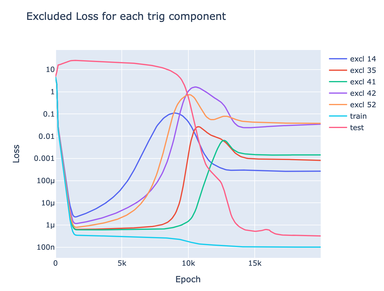
- This is nicely demonstrated by the metric of excluded loss - which roughly shows how much model performance on the training data depends on the generalising algorithm vs memorising algorithm. We see the use of the generalising algorithm to improve training performance rises smoothly over training, well before the grokking point.
Phase Changes
Epistemic status: I feel confident in the empirical results, but the generalisation to non-toy settings is more speculative
Key Takeaways
- Phase changes are surprisingly common
- Empirically, given a problem with a phase change, training it with weight decay and restricted data gives us grokking [AF · GW]
- Speculation: Phase changes occur in any circuit that involves multiple components composing. [AF · GW]
- For example, the composition of the previous token head and the induction head in an induction circuit. The previous token head will only reduce loss if the induction head is there and vice versa. So, initially, the gradients creating each component will be weak to non-existent. But once each component starts to form, the gradients on the other component will become stronger. These effects reinforce each other, and creating a feedback loop that eventually accelerates and results in a phase change.
- Intuitive explanation of grokking [AF · GW]: Regularisation incentivises the model to be simpler, so the model prefers the generalising solution to the memorised solution. The generalising solution is "hard to reach" and the memorising solution is not, so the memorising solution is reached first. But the incentive to find the generalising solution is still there, so the underlying mechanism to induce the phase change is still going on while grokking - memorisation doesn't change this
- Fundamentally, understanding grokking is about understanding phase changes - I don't claim to fully understand phase changes or grokking, but I claim to have reduced my confusion about grokking to my confusion about phase changes.
- Speculation: Phase changes occur for any specific circuit in a model, and so occur all the time in larger models [AF · GW]. Smooth loss curves are actually the average of many small phase changes
- I observe several small phase changes in my toy tasks, eg there's a separate phase change for each digit when learning 5 digit addition.
What Is A Phase Change?
By a phase change, I mean a reverse-S shaped curve[1] in the model's loss on some dataset, or the model's capacity for some specific capability. That is, the model initially has poor performance, this performance plateaus or slowly improves, and suddenly the performance accelerates and rapidly improves (ie, loss rapidly decreases), and eventually levels off.
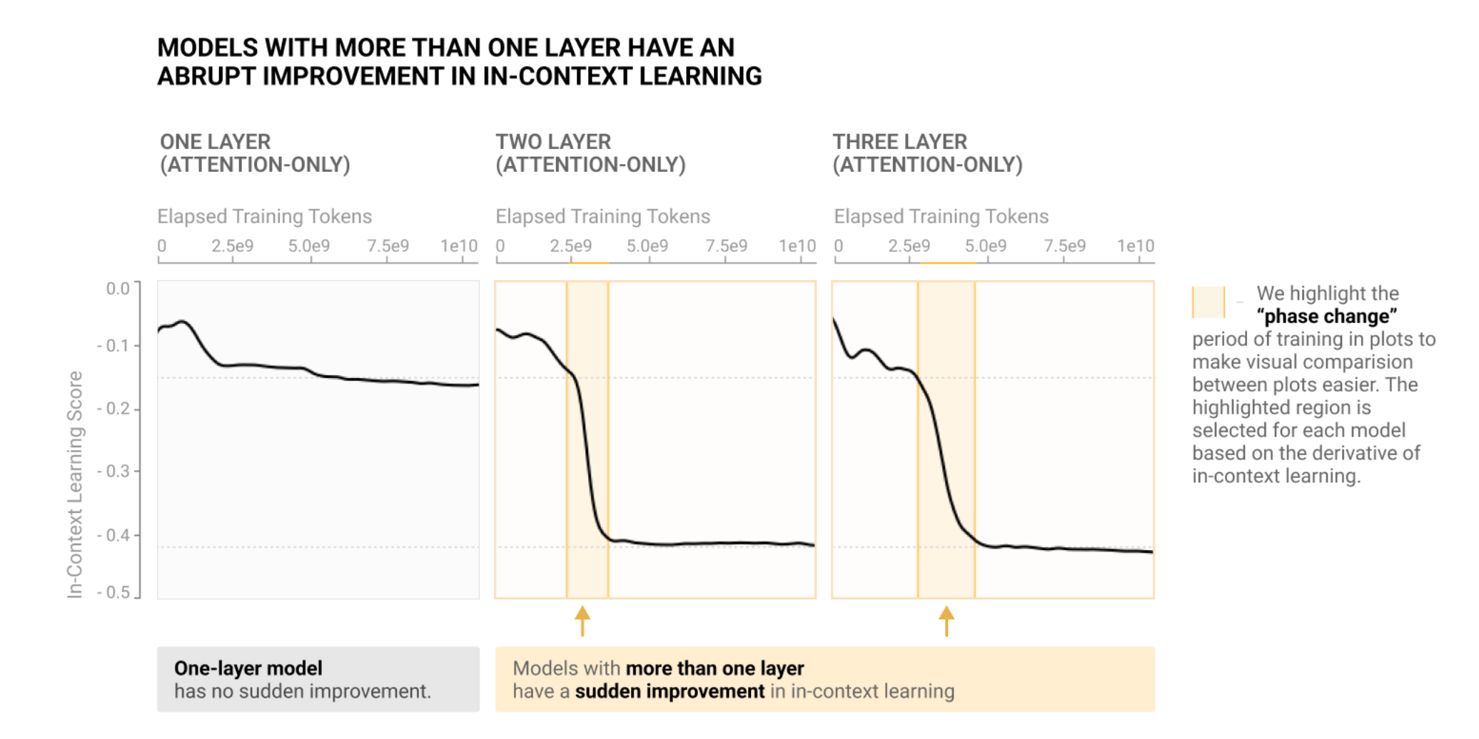
A particularly well-studied motivating example of this is Anthropic's study of induction heads. Induction heads are a circuit in transformers used to predict repeated sequences of tokens. They search the context for previous copies of the current token, and then attend to the token immediately after that copy, and predict that that subsequent token will come next. Eg, if the 3 token surname D|urs|ley is earlier in the context, and the model wants to predict what comes after D, it will attend to urs and predict that that comes next.

The key fact about induction heads are that there is a fairly narrow band of training time where they undergo a phase change, and go from not existing/functional to being fully functional. This is particularly striking because induction heads are the main mechanism behind how Large Language Models do in-context learning - using tokens from far back in the context to usefully predict the next token. This means that there is a clear phase change in a model's ability to do in-context learning, as shown below, and that this corresponds to the formation of a specific circuit via a phase change within the model.
My goal here is to convey the intuition of what I mean by a phase change, rather than give a clear and objective definition. At this stage of research, I favour an informal "I know it when I see it" style definition, over something more formal and brittle.
Empirical Observations
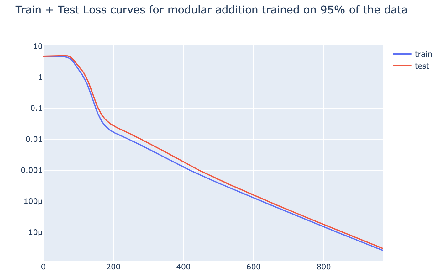
Motivation: Modular addition shows clear grokking on limited data[2], but given much more data it shows a phase change in both train and test loss. This motivated the hypothesis that grokking could be observed any time we took a problem with a phase change and reduced the amount of data while regularising:
In several toy algorithmic tasks I observe phase changes (in both test and train loss) when models are trained on sufficient data[3].
The tasks - see the Colab for more details
- Modular addition mod 113 (1L full transformer)
- Trained on 95% of the training data, 1L Transformer
- 5 digit addition (1L full transformer)
- 1L Transformer, data format
1|3|4|5|2|+|5|8|3|2|1|=|0|7|1|7|7|3 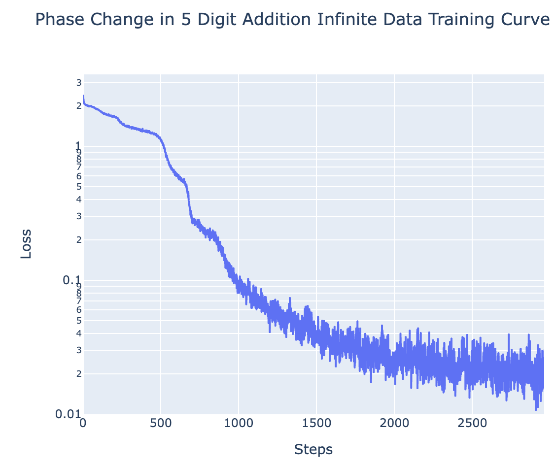
- 1L Transformer, data format
- Predicting Repeated Subsequences (2L attn-only transformer - task designed to need induction heads)
- Data format:
7 2 8 3 1 9 3 8 3 1 9 9 2 5 END- we take a uniform random sequence of tokens, randomly choose a subsequence to repeat, and train the model to predict the repeated tokens. 
- Data format:
- Finding the max element in a sequence (1L attn-only transformer - task designed to need skip trigrams)
- Concretely, the data format is
START 0 4 7 2 4 14 9 7 2 5 3 ENDwith exactly one entry , and the model is trained to output that entry after END. The solution is to learn 10 skip trigrams of the form14 .. END 14 
- Concretely, the data format is
Grokking = Phase Changes + Regularisation + Limited Data
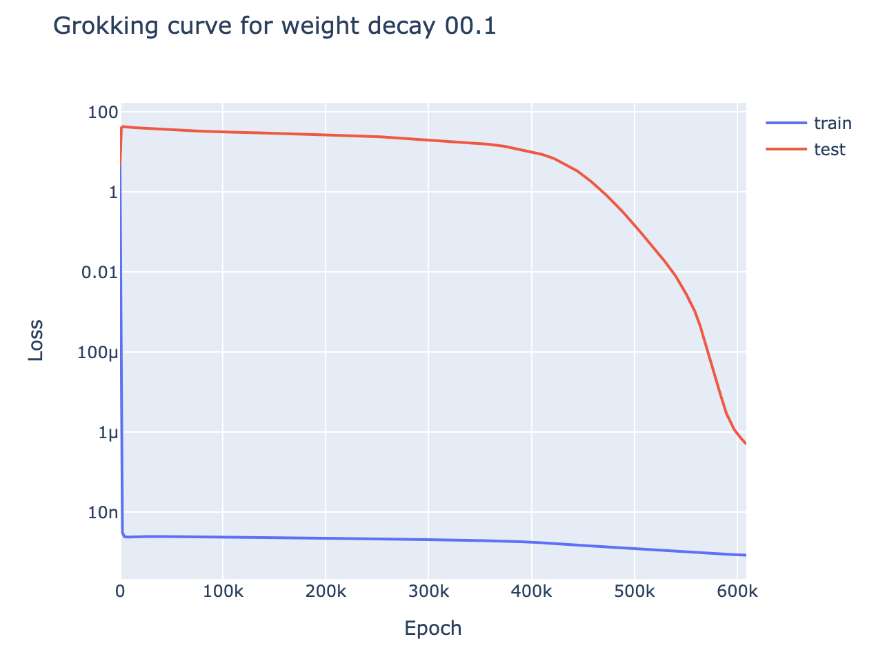
For all of the above tasks, we can induce grokking by adding regularisation (specifically weight decay) and limiting the amount of training data. Eg for 5 digit addition on 700 examples (see the notebook for the rest):
With enough data (eg single epoch training), the model generalises easily, and with sufficiently little data (eg a single data point), the model memorises. But there is a crossover point, and we identify grokking when training with slightly more data than the crossover point - analogous to the findings of Liu et al that grokking is an intermediate state between comprehension and memorisation. I found the crossover points (here, 700) by binary searching by hand. Intuitively, this is consistent with the idea that grokking occurs because of regularisation favouring the simpler solution. Memorisation complexity increases with the amount of data (approximately continuously) while generalising complexity does not, so there should must eventually be a crossover point.
This is particularly interesting, because these tasks are a non-trivial extension of the original grokking. Previous demonstrations of grokking had an extremely small universe of data and were trained on a substantial fraction of it, suggesting that the model may be doing some kind of clever interpolation. While here, the universe of data is much larger (eg possible pairs of 5 digit numbers), and model is trained on a tiny fraction of that, yet it still groks.
Explaining Grokking
Epistemic status: The following two sections are fairly speculative - they're my current best explanation of my empirical findings, but are likely highly incomplete and could easily be totally wrong.
Speculation: Phase Changes Are Inherent to Composition
I recommend reading the section of A Mathematical Framework for Transformer Circuits on Induction Heads to fully follow this section
To understand the link between phase changes and grokking, it's worth reflecting on why circuits form at all. A priori, this is pretty surprising! To see this, let's focus on the example of an induction circuit, and speculate on how it could be formed. The induction circuit is made up of two heads, a previous token head and an induction head, which interact by K-composition. Together, these heads significantly improve loss, but only in the context of the other head being there. Thus, naively, when we have neither head, there should be no gradient encouraging the formation of either head.
At initialisation, we have neither head, and so gradient descent should never discover this circuit. Naively, we might predict that neural networks will only produce circuits analogous to linear regression, where each weight will clearly marginally improve performance as it continuously improves. And yet in practice, neural networks empirically do form sophisticated circuits like this, involving several parts interacting in non-trivial, algorithmic ways.[4]
I see a few different possible explanations for this:
- A lottery ticket hypothesis-inspired explanation:[5] Initially, each layer of the network is the superposition of many different partial circuit components, and the output of each layer is the average of the output of each component. The full output of the network is the average of many different circuits. Some of these circuits are systematically useful to reducing loss, and most circuits aren't. SGD will reinforce the relevant circuits and suppress the useless circuits, so the circuits will gradually form.
- A random walk explanation: The network wanders randomly around the loss landscape, until it happens to get lucky and find a half-formed previous token head and induction head that somewhat compose. Once it has this, this half-formed circuit is useful for reducing loss and gradient descent can take over and make a complete circuit.
- An evolutionary explanation: There's a similar mystery for how organisms develop sophisticated machinery like the human eye, where each part is only useful in the context of other parts. The explanation I find most compelling is that we first developed one component that was somewhat useful on its own, eg a light-detecting membrane. This component was useful in its own right, and so was reinforced, and later components could develop that depend on it, eg the lenses in our eye.
The evolutionary explanation is a natural hypothesis, but we can see from my toy tasks that it cannot be the whole story. In the repeated subsequence task, we have a sequence of uniform randomly generated tokens, apart from a repeated subsequence at an arbitrary location, eg 7 2 8 3 1 9 3 8 3 1 9 9 2 5 END. This means that all pairs of tokens are independent, apart from the pairs of equal tokens in the repeated subsequence. In particular, this means that a previous token head can never reduce loss for the current token - the previous token will always be independent of the next token. So a previous token head is only useful in the context of an induction-like head that completes the circuit. Likewise, an induction head relies on K-composition with a previous token head, and so cannot be useful on its own. Yet the model eventually forms an induction circuit![6]
A priori, the random walk story seems unlikely be sufficient on its own - an induction circuit is pretty complicated, and it likes represents a very small region in model space, and so seems unlikely to be stumbled upon by a random walk[7]. Thus my prediction is that the lottery ticket hypothesis is most of what's going on[8] - an induction head will be useless without a previous token head, but may be slightly useful when composing with, say, a head that uniformly attends to prior tokens, since part of its output will include the previous token! I expect that all explanations are part of the picture though, eg this seems more plausible if the uniform head just so happens to attend a bit more to the previous token via a random walk, etc.
Drawing this back to phase changes, the lottery ticket-style explanation suggests that we might expect to see phase changes as circuits form. Early on in circuit formation, each part of the circuit is very rough, so the effect on the loss of improving any individual component is weak, which means the gradients will be small. But as each component develops, each other component will become more useful, which means that all gradients will increase together in a non-linear way. So as the circuit becomes closer to completion we should expect an acceleration in the loss curve for this circuit, resulting in a phase change.
An Intuitive Explanation of Grokking
With this explanation, we can now try to answer the question of why grokking occurs! To recap the problem setting, we are training our model on a problem with two possible solutions - the memorising algorithm and the generalising algorithm. We apply regularisation and choose a limited amount of data, such that the generalising solution is marginally simpler than the memorising solution[9] and so our training setup marginally prefers the generalising solution over the memorising solution. Naively, we expect the model to learn the generalising solution.
But we are training our model on a problem whose solution involves multiple components interacting to form a complete circuit. So, early in training, the gradients incentivising each component of the generalising solution are weak, because they need the parts to all be formed and lined up properly. Memorisation, however, does not require several components to be lined up in careful and coordinated way[10], so it does not have artificially weak gradients at the start. Thus, at the start, memorisation is incentivised more strongly than generalisation and the model memorises.
So, why does the model shift from memorisation to generalisation? Eventually the training loss plateaus post-memorisation - loss is falling and total weights are rising so eventually the gradients towards lower loss (ie to memorise better) balances with the gradients towards lower weights (ie to be simpler) and cancel out. But they don't perfectly cancel out. If there's a direction in model space that allows it to memorise more efficiently[11], then both gradients will encourage this direction. And the natural way to do this is by picking up on regularities in the data - eg, you can memorise modular addition twice as efficiently by recognising that . This is the same process that leads the model to generalise in the infinite data case - it wants to pick up on patterns in the data.[12]
So the model is still incentivised to reach the generalising solution, just as in the infinite data case. But rather than moving from the randomly initialised model to the generalising model (as in the infinite data case), it interpolates between the memorising solution and the generalising solution. Throughout this process test loss remains high - even a partial memorising solution still performs extremely badly on unseen data! But once the generalising solution gets good enough, the incentive to simplify by deleting the remnants of the memorising solution dominates, and the model clears up the memorising solution, finally resulting in good test performance. Further, as in the infinite data case, the closer we get to the generalising solution the more the rate of change of the loss accelerates. So this final shift happens extremely abruptly - manifesting as the grokking phase change!
As a final bit of evidence, once the model has fully transitioned to the generalising solution it is now inherently simpler, and the point where the incentive to improve loss balances with the incentive to be simpler is marginally lower - we can observe in the graphs here that the model experiences a notable drop in train loss post grokking.
I later walk through this narrative and what it corresponds to in the modular addition case [AF · GW].
Speculation: Phase Changes are Everywhere
My explanation above asserted that phase change are a natural thing to expect with the formation of specific circuits in models. If we buy the hypothesis that most things models do are built up out of many interpretable circuits, then shouldn't we expect to see phase changes everywhere whenever we train models, rather than smooth and convex curves?
My prediction is that yes, we should, and that in fact we do. But that larger models are made up of many circuits and, though each circuit may form in a phase change, the overall loss is made up out of the combination of many different capabilities (and thus many different circuits). And circuits of different complexity/importance likely form at different points in training. So the overall loss curve is actually the sum of many tiny phase changes at different points in training, and this overall looks smooth and convex. Regularities in loss curves like scaling laws may be downstream of statistical properties of the distribution of circuits, which become apparent at large scales. We directly observe the phase change-y ness from the loss curves in these simple toy problems because the problems are easy enough that only one/a few circuits are needed.
Some evidence for this hypothesis:
- 5 digit addition (toy problem) - We can decompose the loss into the sum of 6[13] components - the loss on each of the 6 digits in the sum. When we do this, we observe separate phase changes in each digit, resulting in the many small non-convexities in the overall loss curve.
- The ordering of phase changes is not stable between runs, though token 0 and token 1 tend to be first[14]
- This isn't specific to 5 digit, eg 15 digit addition shows 16 separate phase changes
- Skip Trigrams (toy problem) - The model learns 10 different skip trigrams,
10 .. END 10,11 .. END 11, etc. Each skip trigram shows a separate phase change- Notably, each phase change happens at approximately the same time, so the overall curve looks less bumpy than 5 digit addition. This makes sense, because each skip trigram is "as complex" as the others, while learning to add some digits is much harder than others.
- Induction Heads - Induction heads are the best studied example of a specific circuit through training, and there we see a clear phase change in LLMs up to a 13B transformer. Each head should be "as complex" as the others, so it makes sense that the all occur at approximately, but not exactly, the same time.[15]
- Emergent phenomena - Emergent phenomena are a widely seen thing as language models scale up - they abruptly go from incapable to capable on a task such as addition. As argued by Jacob Steinhardt, More is Different in AI. It seems natural to extend this to a particular model during training, as we know that smaller models trained on more data can outcompete larger models on less data
- AlphaZero Capabilities: One finding in DeepMind's AlphaZero Interpretability paper was that there is a phase change in the model's capabilities, where it learns to represent a lot of chess concepts around step 32,000.
Summary
I think this is highly suggestive evidence that there is a deep relationship between grokking and phase changes, and that grokking occurs when models with a phase change are trained with regularisation and limited data. I present some compelling (to me) explanations of what might be behind the phase change behaviour, and show how this model explains grokking and predicts several specific empirical observations about grokking. I don't claim to fully understand phase changes or grokking, but I do claim to have substantially reduced my confusion about grokking to my confusion about phase changes.
Modular Addition
Epistemic status: I feel pretty confident that I have fully reverse engineered this network, and have enough different lines of evidence that I am confident in how it works. My explanation of how and why it develops during training is shakier.
Key Takeaways
- A 1L Transformer learns a clear and interpretable algorithm to do modular addition. [AF · GW]
- This algorithm operates via using trig identities and Discrete Fourier Transforms to map , and then extracting
- This algorithm can be clearly read off from the weights. If we apply a Discrete Fourier Transform to the input space and apply the Transformer Circuits framework, the structure of the network and its resulting algorithm becomes clear.
- The model naturally forms several sub-networks that calculate the sumn in different frequencies and add these to form the logits. This can be seen by a clear clustering of the neurons
- Within a cluster, individual neurons clearly represent interpretable features for a single frequency.
- To emphasise, this algorithm was discovered purely via gradient descent, not by me. I didn't think of this algorithm until I reverse engineered it from the weights!
- The evolution of this algorithm [AF · GW] can be clearly seen during training, and systematic progress towards the generalising circuit can be seen well before the grokking point
- We can see each phase of my narrative of grokking [AF · GW] manifest during training
- With excluded loss, we can see the model interpolate between memorisation and generalisation. Train loss performance depends substantially on the generalising circuit well before we see a significant change in test loss.
Model Details
In this section I dive deeply into one specific and well-checkpointed model trained to do modular addition. See model training code for more details, but here are the key points:
- The model is trained to map to (henceforth 113 is referred to as )
- 1L Transformer
- Learned positional embeddings
- Width 128
- No LayerNorm
- ReLU activations
- Input format is
x|y|=, where are one-hot encoded inputs, and is an extra token. - Trained with AdamW, with weight decay 1 and learning rate
- Full batch training, trained on 30% of the data (ie the pairs of inputs) for 40,000 epochs[16]
This is a 1L transformer, with no LayerNorm and learned positional embeddings, trained with AdamW with weight decay 1, and full batch training on 30% of the data (the data is the pairs of numbers ). The
Overview of the Inferred Algorithm
The key feature of the algorithm is calculating with - this is a function of and be mapped to , and because has period we get the part for free.
More concretely:
- Inputs are given as one-hot encoded vectors in
- Calculates [AF · GW] via a Discrete Fourier Transform (This sounds complex but is just a change of basis on the inputs, and so is just a linear map)
- , is arbitrary, we just need period dividing
- Calculates [AF · GW] by multiplying pairs of waves in and in
- Calculates [AF · GW] and by rearranging and taking differences
- Calculates [AF · GW] via a linear map to the output logits
- This has an argmax at , so post softmax we're done!
There are a few adjustments to implement this algorithm in a neural network:
- The model's activations at any point are vectors(/tensors). To represent several variables, such as , these are stored as different directions in activation space. When the vector is projected onto those dimensions, the coefficient is the relevant variable (eg )
- The model runs the algorithm in parallel for several different frequencies[17] (different frequencies correspond to different clusters of neurons, different subspaces of the residual stream, and sometimes different attention heads)
Background on Discrete Fourier Transforms
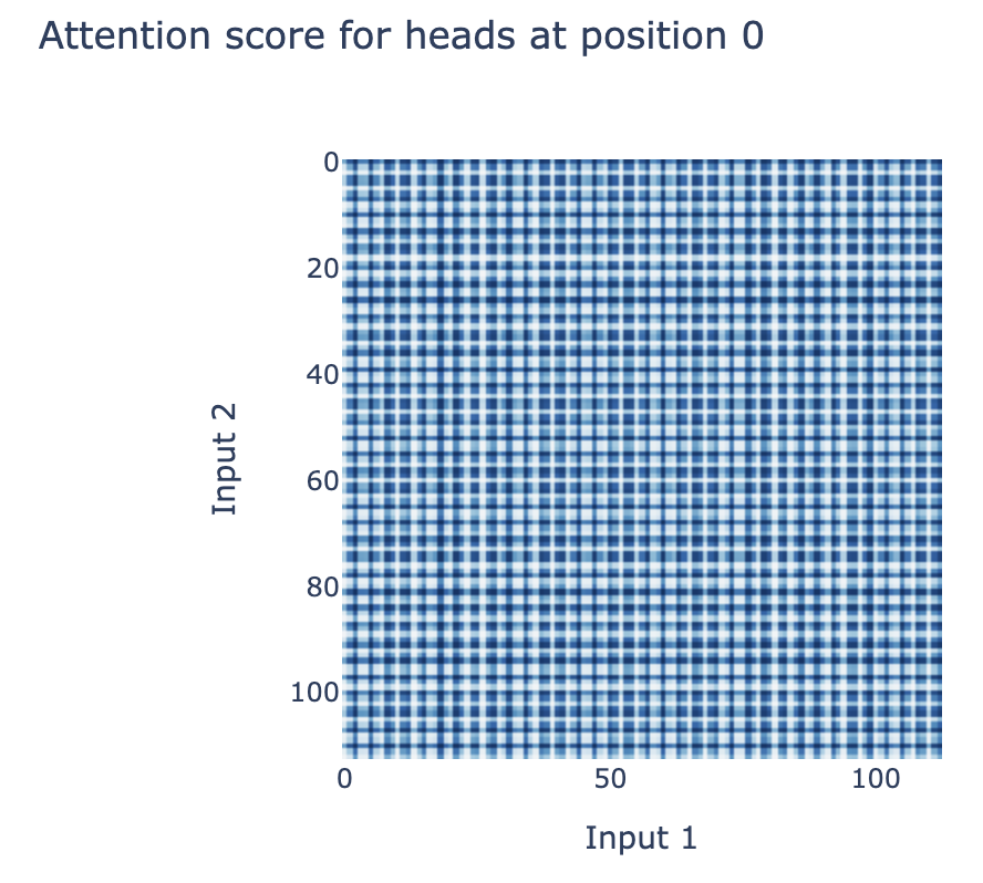
A key technique in all that follows is Discrete Fourier Transforms (DFT). I give a more in-depth explainer in the colab, but here's a rough outline - I expect this requires familiarity with linear algebra to really get your head around. The key motivating observation is that most activations inside the network are periodic and so techniques designed to represent periodic functions nicely are key. Eg the attention patterns:
In , we have a standard basis of the unit vectors. But we can also take a basis of cosine and sine waves, , where is the constant vector, and and are the cosine and sine wave of frequency (henceforth referred to as frequency and represented as for brevity) for . Every pair of waves has dot product zero, unless they're the same wave (ie it's an orthogonal basis). If we normalise these rows, we get an orthonormal basis of cosine and sine waves (so ). We refer to these normalised waves as Fourier Components and this overall basis as the 1D Fourier Basis.
We can apply a change of basis to the 1D input space to , and this turns out to be a much more natural way to represent the input space for this problem, as the network learns to operate in terms of sine and cosine waves. Eg, the fourth column of is the direction corresponding to in the embedding for . If we apply this change of basis to both the input space for and for we apply a 2D DFT, and can represent any function as the linear combination of terms of the form (or , , etc). This is just a change of basis on , and terms of the form (ie the outer product of each pair of rows in ) form an orthogonal basis of vectors (henceforth referred to as the 2D Fourier Basis).
Importantly, this is just a change of basis! If we choose any single activation in the network, this is a real valued function on pairs of inputs , and so is equivalent to specifying a dimensional vector. And we can apply an arbitrary change of basis to this vector. So we can always write it as a linear combination of terms in the 2D Fourier Basis. And any vector of activations is a linear combination of 2D Fourier terms times fixed vectors in activation space. If a function is periodic, this means that it is sparse in the 1D or 2D Fourier Basis, and this is what tells us about the structure of the algorithm and weights of the network.
Reverse Engineering the Algorithm
Here, I present a case for how I was able to reverse engineer the algorithm from the weights. See the Colab and appendices (attention and neuron) for full details, my goal in this section is to roughly sketch what's going on and why I'm confident that this is what's going on.
Calculating waves
Theory: Naively, this seems like the hard part, but is actually extremely easy. The key is that we just need to learn the discretised wave on , not for arbitrary . is input into the network as a one-hot encoded vector, and the multiplied by a learned matrix . We can in fact learn any function [18]
Conveniently, , the matrix of waves , is an orthonormal basis. So will recover the direction of the embedding corresponding to each wave - in other ways, extracting is just a rotation of the input space.
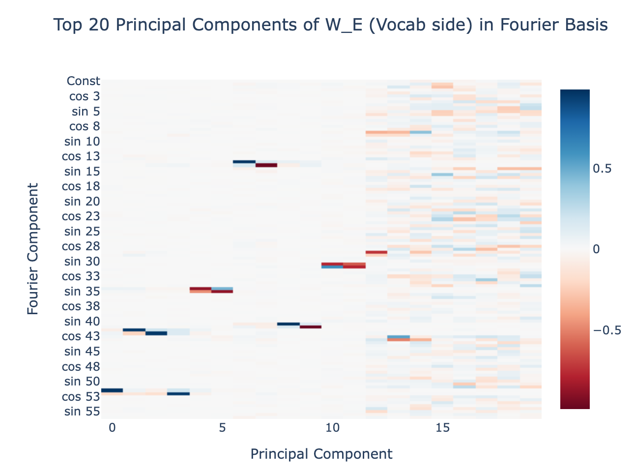
Evidence: We can use the norm of the embedding of each wave to get an indicator of how much the network "cares" about each wave[19], and when we do this we see that the plot is extremely sparse. The model has decided to throw away all but a few frequencies[20]. This is very strong evidence that the model is working in the Fourier Basis - we would expect to see a basically uniform plot if this was not a privileged basis.
Calculating 2D products of waves
Theory: A good mental model for neural networks is that they are really good at matrix multiplication and addition, and anything else takes a lot of effort[21]. As so here! As we saw above, creating is just a rotation, and the later rearranging and map to the logits is another linear map, but multiplying the terms together is hard and non-linear.
There are three non-linear operations in a 1L transformer - the attention softmax, the element-wise product of attention and the value vectors, and the ReLU activations in the MLP layer. Here, the model uses both ReLU activations and element-wise products with attention to multiply terms[22].
The neurons form 5[23] distinct clusters for each frequency, and each neuron in the cluster for frequency has its activation as a linear combination of .[24] Note that, as explained above, the neuron activation in any network can be represented as a linear combination of products of Fourier terms in and Fourier terms in (because they form a basis of ). The surprising fact is that this representation is sparse! This can be visually seen as neuron activations being periodic:
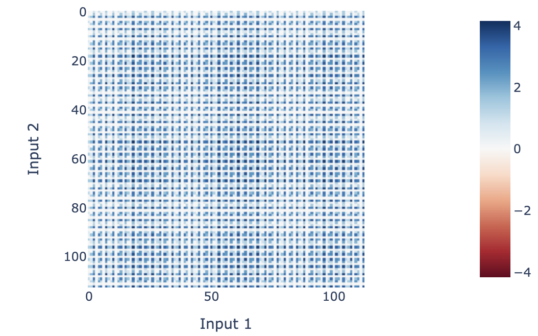
Evidence: The details of how the terms are multiplied together are highly convoluted[25], and I leave them to the Colab notebook appendices. But the neurons do in fact have the structure I described, and this can be directly observed by looking at their values. And thus, by this point in the network it has computed the product terms.
For example, the activations for neuron 0 (as plotted above) are approximately (these coefficients can be calculated by mapping the neuron activation into the 2D Fourier Basis). This approximation explains >90% of the variance in this neuron[26]. We can plot this visually with the following heatmap:
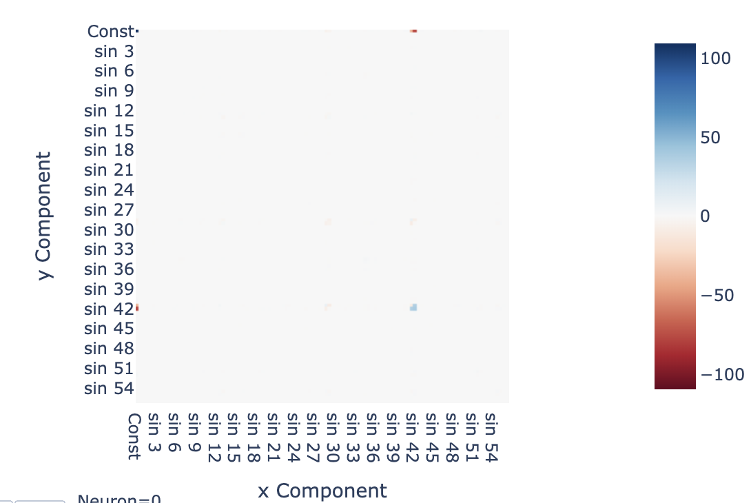
Zooming out, we can apply a 2D DFT to all neuron activations, ie writing all of the neuron activations as a linear combinations of terms of the form times vectors, and plotting the norm of each vector of coefficients. Heuristically, this is telling us what terms are represented by the network at the output of the neurons. We see that the non-trivial terms are in the top row (of the form ) or the left column (of the form ) or in a cell of 2D cells along the diagonal (of the form - notably, a product term where both terms have the same frequency).
Calculating and calculating logits
Theory: The operations mapping and are linear, and the operations mapping this to are also linear. So their composition is linear, and can be represented by a single matrix multiplication. The neurons are mapped to the logits by , and so the effective weight matrix must represent both of these operations (if my hypothesis is correct). Note that is a matrix, mapping from MLP-space to the output space.
Evidence: We draw upon several different lines of evidence here.
We show that the terms are computed as follows: We repeat the above analysis to find terms represented by the neurons on the logits, we find that the terms in the top row and left column cancel out. This leaves just diagonal terms, corresponding to products of waves of the same frequency in x and y, exactly the terms we need. We also see that the 2x2 blocks are uniform, showing that and have the same coefficient. Further analysis shows that everything other than for these 5 frequencies is essentially zero.
We now show that the output logits produce for each of the 5 represented frequencies (where is the term corresponding to the output logits). The neurons form clusters for each frequency, and when we plot the columns of corresponding to those frequencies, and apply a 1D DFT to the output space of , we see that the only non-trivial terms are - ie the output logits coming from these neuron clusters is a linear combination of .
We can more directly verify this by writing approximating the output logits as a sum of and fitting the coefficients . When we do this, the resulting approximated logits explains 95% of the variance in the original logits. If we evaluate loss on this approximation to the logits, we actually see a significant drop in loss, from to
Evolution of Circuits During Training
Note: For this section in particular, I recommend referring to the Colab! That contains a bunch of interactive graphics that I can't include here, where we can observe the development of circuits during training.
Now that we understand what the model is doing during training on a mechanistic level, we can directly observe the development of these circuits during training. The key observation is that the circuits develop smoothly, and make clear and systematic progress towards the generalising circuit well before there is notable test performance. For example, the graph of the norms of the embedding of different waves becomes sparse. In particular, this disproves the natural hypothesis that grokking is the result of a random walk on the manifold of models that perform optimally.
I will now give and explain several graphs of metrics during training, and use them to support my above narrative of what happens during grokking [AF · GW]in this specific case:
- Sum of squared weights - the main regularisation is weight decay, so paying attention to the change in sum of squared weights is key to understand the effect of the regulariser
- This uses the transformer circuits notation - We canare MLP weights, is the unembed, is the embed, are the attention weights
- Excluded loss: Intuitively, this metric tracks how much the model's performance on the training data comes from the generalising algorithm vs the memorisation algorithm, by ablating the model's ability to use a specific frequency . This serves as a progress measure, quantitatively tracking the model's progress towards the correct algorithm.
- Formally, we calculate the logits, use a 2D DFT to write them as a linear combination of waves in x and waves in y, and set the terms corresponding to to zero and keep the other terms the same. Then measure the train loss.
- If the model is using the addition identities (ie, with the generalising algorithm), this will heavily damage performance. If it isn't (ie, the memorising algorithm), then this is just deleting 2 directions among , and so should have no effect.
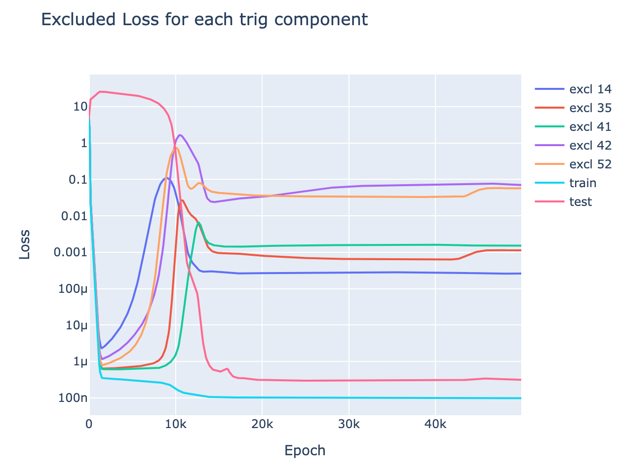
- Formally, we calculate the logits, use a 2D DFT to write them as a linear combination of waves in x and waves in y, and set the terms corresponding to to zero and keep the other terms the same. Then measure the train loss.
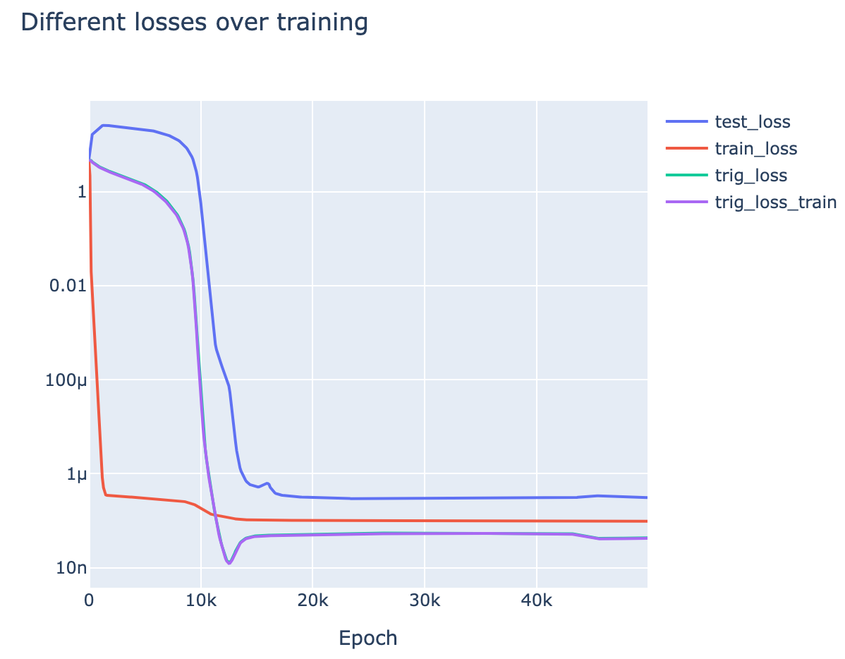
- Trig loss: Another metric is to take the output logits, and only allow them to use the directions corresponding to for the 5 relevant frequencies. Intuitively, this represents the model's performance with the generalising algorithm preserved but the memorising algorithm removed.
- Here we evaluate performance on both the train and test set - trig loss for the train and test set is almost equal (the lines are identical), showing that it's purely tracking the generalising algorithm
We can now use these metrics to analyse the separate stages of training:
- Memorisation (Epoch 0-1K): The model memorises. We see a dramatic drop in train loss, and a rise in test loss.
- We see that the incentive to memorise is far stronger than the incentive to have low weights, as total weights rise a lot
- We see that it's memorising rather than generalising as excluded loss is very close to train loss
- Interpolation (Epoch 1K-9K): The model is interpolating between memorisation and generalisation.
- We see this in the smooth divergence of excluded loss from train loss - this shows that the model is deriving more and more of its training performance from the generalising algorithm.
- Intuitively, the model is trying to memorise "more efficiently" by picking up on patterns in the data. Some directions in neuron space are functions of , namely terms, so it learns to use these directions to represent more and more information.
- Train loss mostly plateaus in this period - this shows that although the model is changing its underlying algorithm, it does this by interpolating between the purely memorising circuit and the purely generalising circuit
- It surprises me that the model can interpolate between two circuits while retaining good performance!
- This stage begins when the incentive for low train loss and the incentive for low weights balance, and train loss abruptly levels out.
- This is particularly clear from epoch 1K-3K, when the weights for the MLP layer drop in norm and meet the other weight matrices. Given a matrix product , we can always scale up and scale down and keep the product the same. The sum of squared weights is minimised when , so all weight matrices between the embed and unembed should have equal norm - this minimises total weights and keeps loss the same. The fact that this does not happen in the first stage shows that the incentive for small weights is too weak and has little effect
- Further, this is suggestive evidence that most of the memorisation comes from changes in the MLP - this matches the hypothesis that memorisation involves "simpler" circuits that don't involve complex composition, and so doesn't need a phase change.
- This is particularly clear from epoch 1K-3K, when the weights for the MLP layer drop in norm and meet the other weight matrices. Given a matrix product , we can always scale up and scale down and keep the product the same. The sum of squared weights is minimised when , so all weight matrices between the embed and unembed should have equal norm - this minimises total weights and keeps loss the same. The fact that this does not happen in the first stage shows that the incentive for small weights is too weak and has little effect
- We see this in the smooth divergence of excluded loss from train loss - this shows that the model is deriving more and more of its training performance from the generalising algorithm.
- Generalisation (Epoch 8K-12K): We see a phase change in trig loss. Trig loss represents "model performance if we delete the memorisation circuit", so this shows that the generalising circuit rapidly develops in a phase change.
- This matches my (admittedly post-hoc) hypothesis that all circuits see phase changes - as each component of the circuit forms, it reinforces the gradients on all other components.
- We further see a rapid acceleration in the decrease in total weights, supporting the idea that there is some cascade as the circuit forms.
- Cleaning Up Noise (Epoch 9K-13K): Somewhat in parallel with the above phase change in trig loss, there is a slightly delayed phase change in test loss. The slight delay indicates that good test loss performance requires both a strong generalising circuit, and the removal of the memorising circuit.
- The rapid removal of the memorisation circuit presumably comes from weight decay - once the memorisation circuit's contribution to loss is low enough, the total weight benefits of removing it outweigh the contribution to loss.
- Stability (Epoch 13K-end)[27]: The model has now transitioned to using the generalising circuit and all our metrics settle down
- The model still has some remnants of the memorisation circuit, as train loss is still less than test loss. This must come from directions other than in logit space, as trig loss is identical on the train and test data.
Discussion
Alignment Relevance
Ultimately, my goal is to do research that is relevant to aligning future powerful AI systems [AF · GW]. Here I've studied tiny models
(Note - the true reason I did this project was that I was on holiday, and got extremely nerd-sniped, so this is all post-hoc reasoning!)
- Emergent capabilities:
- Is grokking relevant to large models? Probably not - models like GPT-3 and PaLM are trained on functionally infinite data, and rarely see a data point twice. In fact, there's a strong incentive to avoid this, as repeated data can severely damage performance.
- The main way I think this is directly relevant to large models is the indication that phase changes are everywhere [AF · GW]. If most circuits emerge as phase changes during training, this suggests we should expect emergent capabilities to be a frequent occurence. In particular, this may occur for particular dangerous capabilities, such as deception or situational awareness [AF · GW]
- This would make alignment a harder problem, as it is less likely that we'll see warning shots. It also limits our ability to, eg, continuously test a system for misalignment or deception throughout training. This strategy might work if the system will first try to be deceptive badly before it is superhuman at lying, but will fail if the system rapidly jumps from not even trying to be deceptive to being superhuman.
- However, this is highly speculative - even if this hypothesis holds, these capabilities may be implemented by many different circuits, and so still see gradual development
- A laboratory for training dynamics + generalisation: There are many open questions about exactly why neural networks work, why they learn to generalise to unseen data, what kinds of generalising algorithms they learn, and how this can be influenced. These are extremely hard questions to study, and I don't feel that I've understood them as a result of this work. But I think the modular addition transformer may be a good laboratory to examine these questions, as it's a concrete, small model that can be easily trained and whose circuits can be clearly inspected. Further, understanding these questions is a key question for alignment - aligning systems will likely require predicting when they would learn to be deceptive vs aligned and how to influence them.
- A particularly important direction may be directly training systems on interpretability-based metrics. Naively, if we could create an automated tool to detect deception and put this in the loss function, our system may never learn to be deceptive. But by default, I would expect this kind of strategy to fail badly, because gradient descent will just find a way to Goodhart the tool. I expect a good (though still highly limited) in-road into this question would be to train the modular addition system on interpretability-based metrics, and see the effects on the training dynamics and the resulting circuits.
- The ability to understand training dynamics rather than just a final system is also notable here. Possibly, if we ever end up with a system that is deceptive and aware of its current situation as a neural network in training [AF · GW], it will be able to influence the training process to always keep it misaligned [AF · GW], and evade any interpretability techniques trying to detect this [AF · GW]. The only way to avoid this will be to influence the training dynamics such that the system never becomes deceptive and situationally aware in the first place.
- Importance of interpretability: A high-level motivation behind this work is a belief that mechanistic interpretability is key to understand how neural networks work. They seem to learn interpretable circuits, and these determine both the model's capabilities, and how those capabilities are implemented. It seems very difficult to get traction on what's really going on in models without engaging with these circuits - analogous to doing chemistry without discovering the periodic table. I take this work as a proof of concept of that - I took the weird and confusing phenomena of grokking, and feel that I have significantly de-mystified it by fully reverse engineering the underlying circuits.
- This is an admittedly very toy problem, but feels like evidence supporting my belief that interpretability extremely useful for getting alignment right [AF · GW].
- This is a particularly notable with grokking, as here we studied the competition between two circuits with comparable loss. The standard way to predict what a model will learn is by expecting it to have low loss, but this breaks down if multiple mechanistically different solutions have comparable performance. This is extremely relevant for alignment as, for example, a deceptive system will be incentivised to output exactly what we'd expect from an aligned solution, and so get the same loss.
- This work also reinforces my belief that the circuits agenda is possible at all - neural networks seem to want to be understood, if we can just find the right way to reverse engineer them! In particular, the fact that I discovered an unexpected and new[28] algorithm for doing modular addition via reverse engineering.
Limitations
There are several limitations to this work and how confidently I can generalise from it to a general understanding of deep learning/grokking, especially the larger models that will be alignment relevant. In particular:
- The modular addition transformer is a toy model, which only needs a few circuits to solve the problem fully (unlike eg an LLM or an image model, which needs many circuits and may lead to different behaviour)
- The model is over-parametrised, as is shown by eg it learning many redundant neurons doing roughly the same task. It has many more parameters than it needs for near-perfect performance on its task, unlike real models.
- In particular, models like language models could always learn more circuits to achieve marginally better task performance, and so need to use their parameters efficiently. This may act as a form of implicit regularisation.
- I only study weight decay as the form of regularisation.
- My explanations of what's going on rely heavily on fairly fuzzy and intuitive notions that I have not explicitly defined: crisp circuits, simplicity, phase changes, what it means to memorise vs generalise, model capacity, etc.
- Of my four tasks exhibiting phase changes, I have only fully interpreted modular addition.[29]
Future Directions
I see a lot of future directions building on this work. If you'd be interested in working on any of these, please reach out! I'd love to chat and possibly advise or collaborate on a project. I'm also currently looking to hire an intern/research assistant to help me work on mechanistically interpretability projects (including but not limited to these ideas), and if you feel excited about any these directions you may be a good fit.
- Investigating the 'phase changes are everywhere' hypothesis.
- Focusing on larger models on complex tasks
- Training a larger model that we know how to interpret, making many checkpoints and inspecting circuits during training
- Training a small SoLU transformer (1L is particularly easy to interpret)
- Training Inception and looking for curve circuits
- Looking for emergent capabilities in open source well-checkpointed training runs (Eg Mistral and GPT-J)
- Performance on benchmarks or specific questions from a benchmark
- Simple algorithmic tasks - eg few shot learning, addition, sorting words into alphabetical order, completing a rhyming couplet, matching open and close brackets
- Soft induction heads, eg translation
- Look at attention heads on various texts and see if any have recognisable attention patterns (eg start of word, adjective describing current word, syntactic features of code like indents or variable definitions, most recent open bracket, etc).
- Wei et al is a good source for other ideas
- Training a larger model that we know how to interpret, making many checkpoints and inspecting circuits during training
- More elaborate toy problems that involve several different tasks
- Eg, training a model with separate heads for modular addition, subtraction, multiplication, etc. Do we see separate phase changes?
- Training models for the other tasks in the grokking paper with more data, and seeing if we see phase changes but no grokking.
- Focusing on larger models on complex tasks
- Investigating the 'phase changes are inherent to composition' hypothesis
- If we directly look at the gradients on different components of the circuit, do we see this mutual reinforcement and cascading?
- Can we show this analytically in some toy setting? What are the minimal properties we need to see phase changes?
- I predict the most tractable will be skip trigrams, given how simple they are. We can take even simpler versions, by making the only parameters a QK and OV matrix, removing the attention softmax, etc.
- Are phase changes specific to weirdnesses of the Adam optimizer? Do we get them for SGD or Momentum?
- Note: Once a model has memorised, loss can be around 1e-7. SGD gradients scale with loss while Adam is normalised, so you'll need to increase your learning rate a lot.
- Barak et al may be another good setting to analyse - looking for phase changes in the k-bit parity problem
- Loose threads in this project
- Interpreting my other tasks with phase changes, and examining the circuits
- Preliminary investigation shows that 5 digit addition is using a variant of the trig based algorithm
- Interpreting the memorisation circuit in the modular addition transformer - understanding memorisation in transformers seems exciting to me!
- This is likely easiest on random labels with no structure.
- Why is there another phase change at epoch 43K?! What's the algorithm after this?
- There's some circuit competition between eg frequency 25 and 31 from epoch 12K to 14K, or between multiplying terms with the attention patterns or the ReLUs. What's up with that?
- Why do the given frequencies form, and not others? Why 5 or 6 frequencies, and not more or less?
- Train the model for a bunch of different random seeds, and see how consistent these observations are.[30]
- Interpreting my other tasks with phase changes, and examining the circuits
- Training dynamics. Note that a 2L MLP can also grok modular addition, and may be easier to study.
- What happens when we train on interpretability-inspired metrics like excluded loss[31]? Can we accelerate the grokking point? Can we disincentivise it? Can we incentivise or disincentivise specific frequencies?
- How do forms of regularisation other than weight decay affect the model and its inductive biases.
- How and why does the model learn to form separate clusters of neurons? Can we predict neuron clustering in advance? Can we manually shift the initialisation to change the clustering?
- Can we replicate a lottery ticket-style approach here? What subnetworks are useful for solving this problem? And if only some subnetworks are useful, why do all neurons ultimately end up being used?
- How general is this algorithm? Can we find Fourier-style algorithms in LLMs? Especially when they learn to do addition
- Note, I expect this to be much easier to detect in models that tokenize each digit separately - the GPT-3 tokenizer completely breaks place value:
28|79|23|598|23|45|987|249|234|0000|23|47|89|03|00000|700|9|02|10. Sadly, the only tokenizer I know of like this is PaLM's. - The GPT-3 tokenizer mostly creates 2 digit tokens, so I'd start by trying to use a linear probe to extract in base 100 from the model for each frequency, where is the correct output digit (or possible the output if you incorrectly carry a 1)
- Note, I expect this to be much easier to detect in models that tokenize each digit separately - the GPT-3 tokenizer completely breaks place value:
Getting into the field: I think this problem is notable for being fairly simple and involving small models that it's tractable to completely understand. If you're interested in getting into mechanistic interpretability and are new to the field, I think this may be a great place to start! As a concrete first project, I recommend training your own transformer for modular subtraction, figuring out the analogous algorithm it should be using, and see if you can replicate my analysis to reverse engineer that.
Meta
Notable Observations
Some scattered thoughts that feel exciting to me, but didn't naturally fit into this write-up:
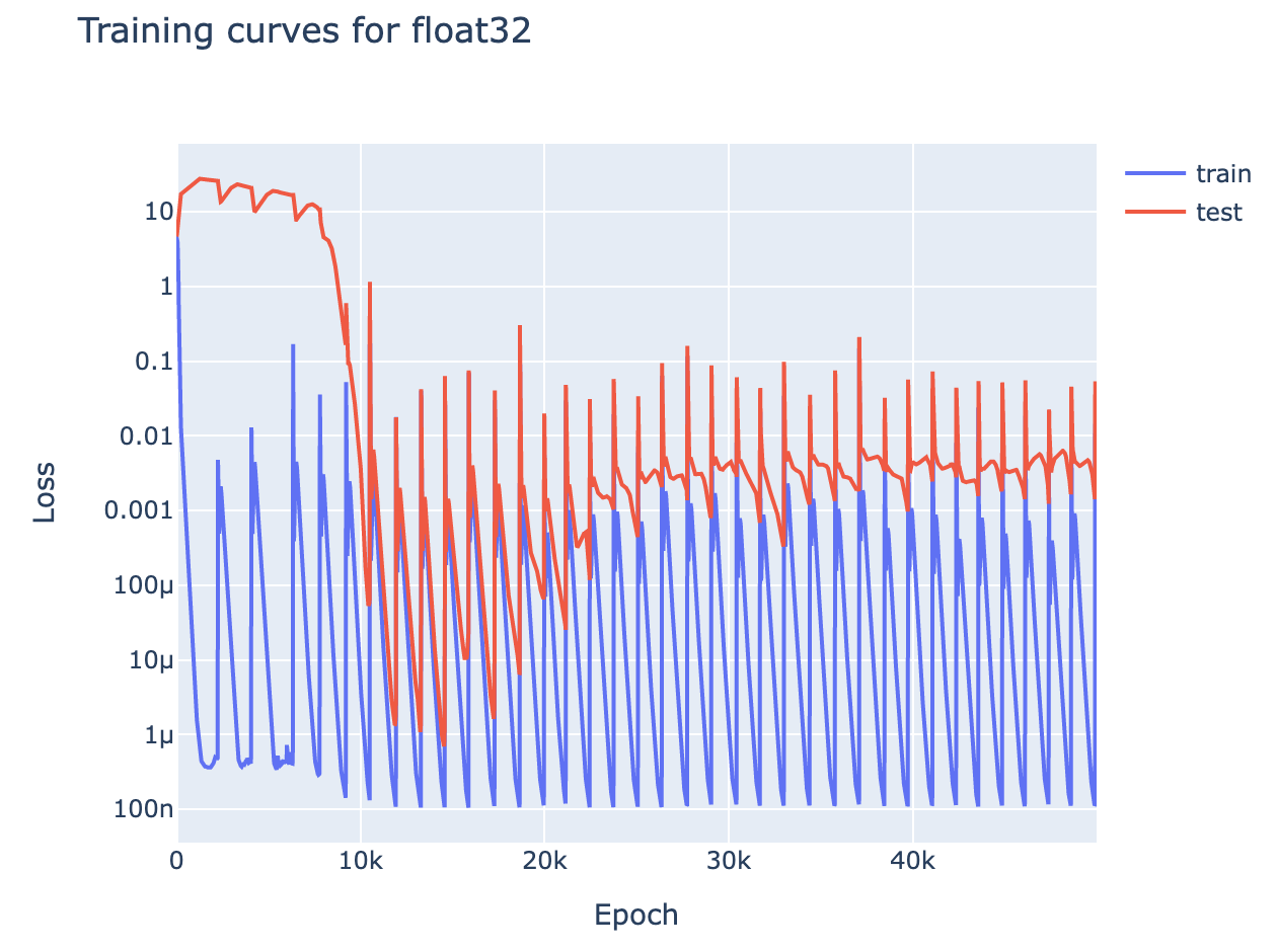
- Slingshot mechanism: (see colab) The Slingshot Mechanism was a fascinating paper from Thilak et al, that found that grokking seemed tied to 'slingshots', dramatic loss spikes, that it was hypothesised flung the model to different regions in the loss landscape.
- I found that these slingshots were not necessary to achieve grokking[32], and further that the slingshots are the result of a float32 precision error in
log_softmax. - This can be fixed by casting your logits to float64 before taking
log_softmax. If I keep my training code exactly the same but remove this casting, my loss curve instead looks like this monstrosity: - Explanation: Concretely, the smallest non-zero value that
log_softmaxcan output in float32 is1.19e-7. So once the model has memorised sufficiently well that loss approaches the scale of1e-7, some data points will have loss rounding to zero. This also rounds the gradients of their loss to zero, equivalent to them not being in the training set. When a model memorises data, it wants to repurpose all other parameters and set unseen data points to extreme values, and this precision error means this includes some training data points. This introduces a dodgy gradient, and the EWMA of Adam ensures it persists for long enough for a significant loss spike- Note that this is an inherent problem of float32, not a flaw in log_softmax. For small values of x,
log_softmax(x)is equal tolog(1+x), and this is approximatelyx.1.19e-7is the smallest value such that1+x!=1in float32. - Float32 isn't the whole story. With minibatch training and float64, we also see loss spikes, though rarer and less severe
- Note that this is an inherent problem of float32, not a flaw in log_softmax. For small values of x,
- I found that these slingshots were not necessary to achieve grokking[32], and further that the slingshots are the result of a float32 precision error in
- Weight Decay: Naively, for a fixed training dataset size, the model should only grok for sufficiently high weight decay. But this is not actually true! Lower weight decay just delays grokking rather than stopping it.
- Intuition: The model will have an incentive to switch to the generalising circuit so long as it has lower total weight than the memorising circuit. Importantly, this holds for any non-zero weight decay. Smaller weight decay just leads to a smaller incentive
- Explaining circle plots of : A notable finding of Liu et al and the original grokking paper is that the embedding matrix of modular addition can be plotted as a circle, by the first two principal components or t-SNE respectively. Now that we understand the underlying circuits, we can see that this clearly follows from the fact that the embedding matrix has orthogonal rows for - these dimensionality reduction techniques are just finding two directions of the same frequency, and observing that a scatter plot of is a circle
- 2L MLPs can grok modular addition: A surprising (to me) result from Liu et al is that a 2L MLP can grok modular addition[33]. I replicated this result, and found that it learned the same algorithm (here, purely using the ReLU/GeLU activations to multiply the waves in x and y). The neurons formed a cluster for every single frequency, with 3-7 neurons per cluster (width 256), and the input and output weights were sparse in the 1D Fourier basis.
Acknowledgements
This work was done as independent research after leaving Anthropic, but benefitted greatly from my work with the Anthropic interpretability team and skills gained, especially from an extremely generous amount of mentorship from Chris Olah. It relies heavily on the interpretability techniques and framework developed by the team in A Mathematical Framework for Transformer Circuits, and a lot of the analysis was inspired by the induction head bump result.
Thanks to Noa Nabeshima for pair programming with me on an initial replication of grokking, and to Vlad Mikulik for pair programming with me on the grokked induction heads experiment.
Thanks to Jacob Hilton, Alex Ray, Xander Davies, Lauro Langosco, Kevin Wang, Nicholas Turner, Rohin Shah, Vlad Mikulik, Janos Kramar, Johannes Treutlein, Arthur Conmy, Noa Nabeshima, Eric Michaud, Tao Lin, John Wentworth, Jeff Wu, David Bau, Martin Wattenberg, Nick Cammarata, Sid Black, Michela Paganini, David Lindner, Zac Kenton, Michela Paganini, Vikrant Varma, Evan Hubinger (and likely many others) for helpful clarifying discussions about this research, feedback, and helping me identify my many ill-formed explanations!
Generously supported by the FTX regrantor program
Author Contributions
Tom Lieberum significantly contributed to the early stages of this project - replicating grokking for modular subtraction, discovering it was possible in a 1L transformer with no LayerNorm, and observing the strongly periodic behaviour of activations and weights
Neel Nanda led the rest of this project - fully reverse engineering the modular addition transformer, analysing it during training, and discovering and analysing the link between grokking and phase changes. He wrote this write-up, and it is written from his perspective.
Feedback
I'd love to hear feedback on this work - parts you find compelling, parts you're skeptical of, parts I explained poorly, cases for why Colab notebooks are a terrible format for papers, etc. You can comment here, or reach me at neelnanda27@gmail.com.
Citation Info
Please cite this work as:
@misc{https://doi.org/10.48550/arxiv.2301.05217,
  doi = {10.48550/ARXIV.2301.05217},

  url = {https://arxiv.org/abs/2301.05217},

  author = {Nanda, Neel and Chan, Lawrence and Lieberum, Tom and Smith, Jess and Steinhardt, Jacob},

  keywords = {Machine Learning (cs.LG), Artificial Intelligence (cs.AI), FOS: Computer and information sciences, FOS: Computer and information sciences},

  title = {Progress measures for grokking via mechanistic interpretability},

  publisher = {arXiv},

  year = {2023},

  copyright = {arXiv.org perpetual, non-exclusive license}
}
- ^
In the ideal case this looks flat, then drops abruptly, then is flat again. In practice, I'm happy to include any striking non-convexities in a curve.
- ^
Ie a divergence in train and test loss
- ^
Where possible, I train the models on infinite data (ie, the data is randomly generated each time, and there are enough possible data points that nothing gets repeated) - in this case I do not distinguish between train and test loss, as train loss is always on unseen data.
- ^
This is even more mysterious when you consider how each head has both an attention (QK) circuit and a value (OV) circuit. The previous token head's QK circuit needs to compose with the positional embeddings and its OV circuit needs to compose with the embedding's output. The induction head's QK circuit needs to compose with the previous token head's output on the K-side, and the embedding on the Q-side, and the OV circuit needs to compose with the embedding and unembedding to be the identity. This is a lot of synchronised and non-trivial interaction! But we know that real networks form circuits with as many moving parts as this, or more, eg curve detecting circuits.
- ^
Eric Michaud gives some evidence for this by finding that, if we project the model's initialised embedding onto the principal components of the final embedding, we still see a circle-like thing - suggesting that the model reinforced directions in embedding space that luckily had good properties.
- ^
I have not verified that the model actually forms an induction circuit of the form described in this particular task. But the structure of attention means it must be doing some kind of composition, because a single attention head cannot attend to a previous token based on its neighbours
- ^
I later show in the case of modular addition that it is definitively not a random walk, as we can see clear progress towards the true answer before grokking
- ^
Though I'm sure I'm missing other explanations!
- ^
This is a more complex statement than it looks, since each solution can always become more complex to result in lower loss. Eg doubling will always decrease loss if there's 100% accuracy. I operationalise this as 'which solution is simpler if we set them both to achieve the same level of loss'
- ^
I am assuming this fact about memorisation as part of this story. I don't understand how memorisation is implemented so I cannot be confident, but this seems plausible given that, eg a logistic/linear regression model with enough parameters can memorise random data
- ^
ie, more simply/with lower total weights
- ^
In some sense, single epoch training is the limiting case of this. The model tries to memorise every data point it sees, but there must eventually be a cap on how much data it can memorise, so it must pick up on patterns. We never run the model on the same data point twice, so we don't notice this attempt at memorisation. Plausibly, models that never learn to generalise keep trying to memorise recent training data and forget about old data.
- ^
The 0th digit is the leading digit that's 0 or 1
- ^
This is weird! Token 5 (the final digit) should be easiest because it never requires you to carry a 1 - it's just addition mod 10
- ^
Under this hypothesis, I would predict that soft induction heads like translation appear after the phase change, as they seem likely more complex
- ^
The training run was up to 50K epochs, but there's a mysterious bonus tiny phase change at epoch 43K that I don't yet understand, and so I snap the model before then, as I don't think that shift is central to understand the first grok.
- ^
This is useful because, though is an argmax of , the difference between it and the second largest value is tiny. While if we take the sum of for several different values of , the waves constructively interfere at , and destructively interfere everywhere else, significantly increasing the difference.
- ^
By having a column of be - the dot product (ie the first coordinate of the embedding) is . In fact, so long as is invertible, we can recover any function by projecting onto the direction
- ^
Remember that we're using high weight decay, so the model will set any weights it's not using to (almost) zero
- ^
The frequencies here are - as far as I can tell, the specific frequencies and the number of frequencies are arbitrary, and vary between random seeds
- ^
But is also extremely necessary! Eg how activation functions take an MLP from linear regression to being able to represent any function.
- ^
The attention pattern multiplication is the obvious way to do it - I found the use of ReLUs very surprising! But it turns out that is approx (more details)
- ^
The model calculates 6 frequencies with the embedding, but only 5 with the neurons - I'm not sure why.
- ^
There is actually a sixth cluster not aligned with any particular frequency - neurons in this cluster always fire, and thus ReLU is the identity. I'm not entirely sure why this is useful to the network
- ^
In particular, understanding ReLU in the Fourier basis takes it from a nice basis aligned operation to the operation "rotate out of the Fourier basis into the standard basis, take the elementwise ReLU, and then rotate back into the Fourier basis"
- ^
We can validate that the remaining 10% is just noise by ablating - replacing each neuron by this approximation (ie removing all terms of all other frequencies) leaves loss unchanged.
- ^
This isn't quite true - at epoch 43K, there is a tiny phase change which can be seen if you zoom in on the trig loss graph (trig loss and train loss fall, test loss rises). I haven't investigated this properly, but the model goes from never attending to the
=token to significantly attending to it. Presumably there's some further circuit development here? - ^
Well, new to me - ancedotally, a friend of mine came up with the algorithm independently when exploring grokking
- ^
Though skip trigrams are extremely easy to interpret, and mostly match what I'd predict, I just haven't written it up.
- ^
I've looked at several models, but not exhaustively
- ^
Note that excluded loss specifically is weird, because we fit the coefficients of to the logits across all of the data, so it's technically also a function of the test data. Probably linear regression on just the train logits would suffice though.
- ^
Though plausibly helps by adding regularisation - generalising solution may be more stable to slingshots than memorised ones?
- ^
Input format is the sum of a one-hot encoding of x and of y in . If then the vector has a single two in it.
48 comments
Comments sorted by top scores.
comment by Neel Nanda (neel-nanda-1) · 2023-12-31T14:03:31.459Z · LW(p) · GW(p)
Self-Review: After a while of being insecure about it, I'm now pretty fucking proud of this paper, and think it's one of the coolest pieces of research I've personally done. (I'm going to both review this post, and the subsequent paper). Though, as discussed below, I think people often overrate it.
Impact The main impact IMO is proving that mechanistic interpretability is actually possible, that we can take a trained neural network and reverse-engineer non-trivial and unexpected algorithms from it. In particular, I think by focusing on grokking I (semi-accidentally) did a great job of picking a problem that people cared about for non-interp reasons, where mech interp was unusually easy (as it was a small model, on a clean algorithmic task), and that I was able to find real insights about grokking as a direct result of doing the mechanistic interpretability. Real models are fucking complicated (and even this model has some details we didn't fully understand), but I feel great about the field having something that's genuinely detailed, rigorous and successfully reverse-engineered, and this seems an important proof of concept. IMO the other contributions are the specific algorithm I found, and the specific insights about how and why grokking happens. but in my opinion these are much less interesting.
Field-Building Another large amount of impact is that this was a major win for mech interp field-building. This is hard to measure, but some data:
- There are multiple papers I like that are substantially building on/informed by these results (A toy model of universality, the clock and the pizza, Feature emergence via margin maximization, Explaining grokking through circuit efficiency
- It's got >100 citations in less than a year (a decent chunk of these are semi-fake citations from this being used as a standard citation for 'mech interp exists as a field', so I care more about the "how many papers would not exist without this" metric)
- It went pretty viral on Twitter (1,000 likes, 300,000 views)
- This was the joint first mech interp paper at a top ML conference (ICLR 23 spotlight) and seemed to get a lot of interest at the conference.
- Anecdotally, I moderately often see people discussing this paper, or who know of me from this paper
- At least one of my MATS scholars says he got into the field because of this work.
Is field-building good? It's plausible to me that, on the margin, less alignment effort should be going into mech interp, and more should go into other agendas. But I'm still excited about mech interp field building, think this is a solid and high-value thing, and that field-building is often positive sum - people often have strong personal fits to different areas, and many people are drawn to it from non-alignment motivations. And though there's concern over capabilities externalities, my guess is that good interp work is strongly net good.
Is it worth publishing in academic venues Submitting this to ICLR was my first serious experience with peer review. I'm not sure what updates I've made re whether this was worth it. I think some, but probably <50% of the field-building benefit came from this, and that going Twitter viral was much more important for ensuring people became aware of the work. I think it made the work more legitimate-seeming, more citable, more respectable, etc. On an object level, it resulted in the writing, ideas and experiments becoming much better and clearer (though led to some of the more interesting speculation being relegated to appendix E :'( ) though this was largely due to /u/lawrencec 's skills. I definitely find peer review/conforming to academic conventions very tedious and irritating, and am very grateful to Lawrence for doing almost all of the work.
Personal benefit It's hard to measure, but I think this turned out to be substantially good for my career, reputation and influence. It's often been what people know me for, and I think has helped me snowball into other career successes.
Ways it's overrated As noted, I do think there's ways people overrate the results/ideas here, and that there's too much interest in the object level results (the Fourier Multiplication algorithm, and understanding grokking). Some thoughts:
- The specific techniques I used to understand the model are super specific to modular addition + Fourier stuff, and not very useful on real models (though I hold out hope that it'll be relevant to how language models do addition!)
- People often think grokking is a key insight about how language models learn, I think this can be misleading. Grokking is a fragile and transitionary state you get when your hyper-parameters are just right (a bit more or less data makes it memorise or generalise immediately) and requires a ton of overtraining on the same data gain and again. I think grokking gives some hints that individual circuits may be learned in sudden phase transitions (the quantization model of neural scaling), but we need much more evidence from real models on these questions. And something like "true reasoning" is plausibly a mix of many circuits, each with their own phase transition, rather than a thing that'll be suddenly grokked.
- People often underestimate the difficulty jump in interpreting real models (even a 1L language model) compared to the modular addition model, and get too excited about how easy it'll be
- People also get excited about more algorithmic interp work. I think this is largely played out, and focus on real models in my own work (and the work I supervise). I ultimately care about reverse-engineering AGI, and I think language models (even small ones) are decent proxies for this, while algorithmic problem models are not, unless you set up a really good one, that captures some property of real models that we care about. And I'm unconvinced there's much more marginal value in demonstrating that algorithmic mech interp is possible.
comment by dsj · 2022-08-18T02:41:08.240Z · LW(p) · GW(p)
[Edit Jan 19, 2023: I no longer think the below is accurate. My argument rests on an unstated assumption: that when weight decay kicks in, the counter-pressure against it is stronger for the 101th weight (the "bias/generalizer") than the other weights (the "memorizers") since the gradient is stronger in that direction. In fact, this mostly isn't true, for the same reason Adam(W) moved towards the solution to begin with before weight decay strongly kicked in: each dimension of the gradient is normalized relative to its typical magnitudes in the past. Hence the counter-pressure is the same on all coordinates.
A caveat: this assumes we're doing full batch AdamW, as opposed to randomized minibatches. In the latter case, the increased noise in the "memorizer" weights will in fact cause Adam to be less confident about those weights, and thus assign less magnitude to them. But this happens essentially right from the start, so it doesn't really explain grokking.
Here's an example of this, taking randomized minibatches of size 10 (out of 100 total) on each step, optimizing with AdamW (learning rate = 0.001, weight decay = 0.01). I show the first three "memorizer" weights (out of 100 total) plus the bias:

As you can see, it does place less magnitude on the memorizers due to the increased noise, but this happens right from the get-go; it never "groks".
If we do full batch AdamW, then the bias is treated indistinguishably:

For small weight decay settings and zero gradient noise, AdamW is doing something like finding the minimum-norm solution, but in space, not space.]
Here's a straightforward argument that phase changes are an artifact of AdamW and won't be seen with SGD (or SGD with momentum).
Suppose we have 101 weights all initialized to 0 in a linear model, and two possible ways to fit the training data:
The first is . (It sets the first 100 weights to 1, and the last one to 0.)
The second is . (It sets the first 100 weights to 0, and the last one to 1.)
(Any combination with will also fit the training data.)
Intuitively, the first solution memorizes the training data: we can imagine that each of the first 100 weights corresponds to storing the value of one of the 100 samples in our training set. The second solution is a simple, generalized algorithm for solving all instances from the underlying data distribution, whether in the training set or not.
has an norm which is ten times as large as . SGD, since it follows the gradient directly, will mostly move directly toward as it's the direction of steeper descent. It will ultimately converge on the minimum norm solution . (Momentum won't change this picture much, since it's just smearing out each SGD step over multiple updates, and each individual SGD step goes in the direction of steepest descent.)
AdamW, on the other hand, is basically the same as Adam at first, since weight decay doesn't do much when the weights are small. Since Adam is a scale-invariant, coordinate-wise adaptive learning rate algorithm, it will move at the same speed for each of the 101 coordinates in the direction which reduces loss, moving towards the solution , i.e. with heavy weight on the memorization solution. Weight decay will start to kick in a bit before this point, and over time AdamW will converge to (close to) the same minimum-norm solution as SGD. This is the phase transition from memorization to generalization.
Replies from: jacob_cannell↑ comment by jacob_cannell · 2022-08-19T06:56:59.222Z · LW(p) · GW(p)
This is a straightforward argument to test this idea/argument!
I think you may be correct in that regular SGD has an implicit L2 simplicity prior that Adam family optimizers trade for the more important robustness at speed (regular SGD is just completely wrong and fails hard for many compute graphs that don't fit the restrictive zero mean zero variance statistics assumptions). And AdamW with weight complexity prior behaves differently enough that the phase transitions could be specific to AdamW.
But maybe not? Even with pure SGD, you can get nonlinear dynamics through increasing depth (trivial example, consider a deep network of stacked repeated layers - the gradient updates become increasingly multiplicative/lognormal with depth rather than additive/normal).
Replies from: dsj↑ comment by dsj · 2022-08-19T10:38:49.637Z · LW(p) · GW(p)
I agree with you that that’s possible under some conditions and that my argument is not a proof. I note, however, that for the large neural networks used today, there’s theory and evidence (at least under SGD) supporting the idea that they’re effectively approximately linear models (that is, linear in their weights, not linear in their inputs), because the higher-order (multiplicative) effects you describe don't matter since total weight updates throughout training are small. (Actually, I suspect the proof doesn't hold for Adam.)
Even in the case of a nonlinear model, SGD has, as you say, an implicit prior for small movements as measured by the norm, whereas Adam has an implicit prior for small movements as measured by the norm, but then as weight decay becomes more significant throughout training, you start to get this competition from the norm, and once you interpolate the training data, that becomes all you care about.
It's worth noting further that the volume of an ball of a given constant radius increases much faster with dimension than the volume of an ball. This implies that the effective capacity of a high-parameter network trained by Adam for N steps is much larger than that same network trained by SGD for N steps with a comparable or smaller learning rate and gradient not too large (these assumptions typically hold). Thus, the "small movement" prior of Adam is barely a simplicity prior at all, in relative terms.
Replies from: jacob_cannell↑ comment by jacob_cannell · 2022-08-19T18:45:57.588Z · LW(p) · GW(p)
The "large ANNs are effectively linear" predicts that the brain would be even more linear, as it is far wider. And indeed there is some interesting indirect evidence supporting that - at the infinite width limit full backprop becomes unnecessary and equivalent to simpler feedback alignment models. This ties in nicely with that research track trying to explain how the brain learns using SGD like optimization sans backprop.
But on the other hand this linear-limit neural tangent model only applies for simple networks, which are pretty limited. I'll define complex networks as those which have multiplicative interactions in the forward pass. Attention/routing, short/medium term memory, gating etc are all computationally equivalent in their general forms, and all require multiplicative interactions in the forward pass (ie the transpose multiply enabling sequence memory/attention in transformers).
Multiplicative non-linearity seems necessary for high capability/efficiency but also makes training dynamics non-linear - small changes in hidden state (and thus weights) can amplify to very large effects in outptuts/gradients etc. (With sparse memory operations being the extreme example of maximally efficient and maximally nonlinear)
Replies from: dsj↑ comment by dsj · 2022-08-19T19:09:43.483Z · LW(p) · GW(p)
Hmm, I think I understand what you’re pointing at but it’s not obvious to me that the conclusion is correct. If I wear my “infinite hidden width extremist” hat, I’d say that the network after training has extremely similar hidden activations on input x as the network before training. It’s just that the hidden activations have moved in a coordinated way so as to make the output layer come out very differently.
So yeah, the nonlinearities are all there, but they’re fixed nonlinearities of hidden features, and the network’s job is to learn the right linear combination of those fixed nonlinear features.
I’m not confident that this will hold in transformer networks, but I’m not confident it won’t either. Keep in mind that MLPs can learn to multiply, but (if sufficiently wide) they’re still effectively linear models. So the mere existence of nonlinear, multiplicative interactions as a function of the input doesn’t guarantee nonlinearity in the weights.
Replies from: jacob_cannell↑ comment by jacob_cannell · 2022-08-19T19:36:21.004Z · LW(p) · GW(p)
MLPs learning to multiply binary digits is mostly unrelated. The difference I am talking about (simple linear vs complex non-linear) is perhaps better illustrated by considering networks with exponent activation functions rather than relu. Relu is by-design about as close to linear as one can get while still being useful. With exp activation functions the outputs/gradients are rather obviously non-linear in weights.
Another example again is extreme activation sparsity through k-max hidden layers with low k.
Replies from: dsj↑ comment by dsj · 2022-08-19T20:02:49.112Z · LW(p) · GW(p)
MLPs can learn to multiply general real numbers, not just binary digits, so long as the inputs are bounded. I’m actually not clear on why that example is mostly unrelated. It illustrates that you can have an arbitrary nonlinear circuit in part of the network while still being effectively linear in terms of weights, due to the weights staying in a small neighborhood of initialization. It’s actually not at all obvious to me that exponential activation functions would ruin this property. In fact I suspect they don’t in the infinite width limit, although that infinite width limit might be a worse approximation in practice.
Note that the question is ultimately not whether the network is truly linear in weights, but whether it’s effectively linear in weights over the range they move in. A nonlinear smooth function can be usefully treated as linear if we constrain ourselves to a small enough neighborhood. What’s not obvious to me is whether this approximation works for transformers. I wouldn’t be surprised either way.
comment by wesg (wes-gurnee) · 2022-08-17T02:41:23.646Z · LW(p) · GW(p)
Could you describe your inner thought loop when conducting these sorts of mechanistic analyses? I.e., What Are You Tracking In Your Head? [LW · GW]
comment by aysja · 2022-08-25T07:11:43.331Z · LW(p) · GW(p)
I love this work! It’s really cool to see interpretability on toy models in such a clear way.
The trend from memorization to generalization reminds me of the information bottleneck idea. I don’t know that much about it (read this Quanta article a while ago), but they appear to be making a similar claim about phase transitions. I believe this is the paper one would want to read to get a deeper understanding of it.
comment by Gunnar_Zarncke · 2022-08-15T13:27:58.325Z · LW(p) · GW(p)
You don't talk about human analogs of grokking, and that makes sense for a technical paper like this. Nonetheless, grokking also seems to happen in humans, and everybody has had "Aha!" moments before. Can you maybe comment a bit on the relation to human learning? It seems clear that human grokking is not a process that purely depends on the number of training samples seen but also on the availability of hypotheses. People grok faster if you provide them with symbolic descriptions of what goes on. What are your thoughts on the representation and transfer of the resulting structure, e.g., via language/token streams?
Replies from: neel-nanda-1, jacob_cannell↑ comment by Neel Nanda (neel-nanda-1) · 2022-08-15T17:08:25.821Z · LW(p) · GW(p)
Hmm. So firstly, I don't think ML grokking and human grokking having the same name is that relevant - it could just be a vague analogy. And I definitely don't claim to understand neuroscience!
That said, I'd guess there's something relevant about phase changes? Internally, I know that I initially feel very confused, then have some intuition of 'I half see some structure but it's super fuzzy', and then eventually things magically click into place. And maybe there's some similar structure around how phase changes happen - useful explanations get reinforced, and as explanations become more useful they become reinforced much faster, leading to a feeling of 'clicking'
It seems less obvious to me that human grokking looks like 'stare at the same data points a bunch of times until things click'. It also seems plausible that there's some transfer learning going on - here I train models from scratch, but when I personally grok things it feels like I'm fitting the new problem into existing structure in my mind - maybe analogous to how induction heads get repurposed for few shot learning
Replies from: rodrigo-heck-1↑ comment by Rodrigo Heck (rodrigo-heck-1) · 2022-08-16T18:47:01.987Z · LW(p) · GW(p)
It seems less obvious to me that human grokking looks like 'stare at the same data points a bunch of times until things click'
Personally, I don't think it's that different. At least for language. When I read some unrecognizable word in a foreign language, my mind tries first to retrieve other times I have seen this word but haven't understood. Suppose I can remember 3 of these instances. Now I have 3 + 1 of these examples in my mind and, extracting the similar context they share, I can finally deduct the meaning.
↑ comment by jacob_cannell · 2022-08-19T07:04:05.573Z · LW(p) · GW(p)
I have a distinct strong memory of grokking at a very young age (naturally well before I heard the term), learning the basic idea of base-10 digit increments from a long list of the integer sequence examples. What I find most interesting is how rewarding grokking is. There's this clear strong aha! reward feeling in the brain when one learns a low complexity rule that compresses some (presumably important) high level sensory token stream.
There's a pretty strong bayesian argument that learning is sensory compression and so this is just the general low level mechanism underlying much of the brain, but at the same time it seems to have a high level system 2 counterpart.
comment by Daniel Kokotajlo (daniel-kokotajlo) · 2022-08-16T17:39:50.428Z · LW(p) · GW(p)
Thanks, this is awesome! Especially cool that you were able to reverse-engineer the learned algorithm! And the theory/analysis seems great too.
[Just thinking aloud my confusion, not important] --Not sure I understand the difference between random walk hypothesis and lottery ticket inspired hypothesis. In both cases there's a phase transition caused by accelerating gradients once weak versions of all the components of the nonmodular circuit are in place. --The central piece of evidence you bring up is what exactly... that the effectiveness of the nonmodular circuit rises before the phase transition begins. I guess I'm a bit confused about how this works. If I imagine a circuit consisting of a modular memorized answer part and another part, the generalizing bit, that actually computes the answer... if the second part is really crappy/weak/barely there, I don't see how making it stronger is incentivised. Making it stronger means more weights so the regularization should push against it, UNLESS you can simultaneously delete or dampen weights from the memorized answer part, right? But because the generalizing part is so weak, if you delete or dampen weights from the memorized answer part, won't loss go up? Because the generalizing part isn't ready yet to take over the job of the memorized answers?
Replies from: neel-nanda-1, neel-nanda-1, jacob_cannell, jacob_cannell↑ comment by Neel Nanda (neel-nanda-1) · 2022-08-17T06:15:52.015Z · LW(p) · GW(p)
Thanks! I agree that they're pretty hard to distinguish, and evidence between them is fairly weak - it's hard to distinguish between a winning lottery ticket at initialisation vs one stumbled upon within the first 200 steps, say.
My favourite piece of evidence is [this video from Eric Michaud](https://twitter.com/ericjmichaud_/status/1559305105521926144) - we know that the first 2 principle components of the embedding form a circle at the end of training. But if we fix the axes at the end of training, and project the embedding at the start of training, it's pretty circle-y
↑ comment by Neel Nanda (neel-nanda-1) · 2022-08-17T06:18:07.845Z · LW(p) · GW(p)
Making it stronger means more weights so the regularization should push against it, UNLESS you can simultaneously delete or dampen weights from the memorized answer part, right?
I think this does happen (and is very surprising to me!). If you look at the excluded loss section, I ablate the model's ability to use one component of the generalising algorithm, in a way that shouldn't affect the memorising algorithm (much), and see the damage of this ablation rise smoothly over training. I hypothesise that it's dampening memorisation weights simulatenously, though haven't dug deep enough to be confident. Regardless, it clearly seems to be doing some kind of interpolation - I have a lot of progress measures that all (both qualitatively and quantitatively) show clear progress towards generalisation pre grokking.
↑ comment by jacob_cannell · 2022-08-16T21:17:30.738Z · LW(p) · GW(p)
A maximally sparse neural net layer (k=1 max, only one neuron active) effectively is just a simple input->output key/value map and thus can only memorize. It can at best learn to associate each input pattern with one specific output pattern, no more, no less (and can perfectly trivial overfit any dataset of N examples by using N neurons and NI + NO memory, just like a map/table in CS).
We can get some trivial compression if there are redundant input-> output mappings, but potentially much larger gains by slowly relaxing that sparsity constraint and allowing more neurons to be simultaneously active to provide more opportunities to compress the function. With k=2 for example and N=D/2, each neuron now responds to exactly two different examples and must share the input->output mapping with one other neuron - by specializing on different common subset patterns for example.
At the extreme of compression we have a neural circuit which computes some algorithm that fits the data well and is likely more dense. In the continuous circuit space there are always interpolations between those circuits and memorization circuits.
↑ comment by jacob_cannell · 2022-08-16T21:00:10.206Z · LW(p) · GW(p)
The training path is always continuous, thus it necessarily interpolates smoothly between some overfit memorization and the generalizing (nonmodular) circuit solution. But that shouldn't be too surprising - a big circuit can always be recursively decomposed down to smaller elementary pieces, and each elementary circuit is always logically equivalent to not a single unique lookup table, but an infinite set of overparameterized equivalent redundant lookup tables.
So it just has to find one of the many redundant lookuptable (memorization) solutions first, then smoothly remove redundancy of the lookup tables. The phase transitions likely arise due to semi-combinatoric dependencies between layers (and those probably become more pronounced with increasing depth complexity).
comment by gwern · 2023-01-16T20:50:47.421Z · LW(p) · GW(p)
Possibly also of interest: https://cprimozic.net/blog/reverse-engineering-a-small-neural-network/
comment by orthonormal · 2022-09-12T00:45:25.673Z · LW(p) · GW(p)
This is honestly some of the most significant alignment work I've seen in recent years (for reasons I plan to post on shortly), thank you for going to all this length!
Typo: "Thoughout this process test loss remains low - even a partial memorising solution still performs extremely badly on unseen data!", 'low' should be 'high' (and 'throughout' is misspelled too).
Replies from: neel-nanda-1↑ comment by Neel Nanda (neel-nanda-1) · 2022-09-12T01:06:18.134Z · LW(p) · GW(p)
Thanks, I really appreciate it. Though I wouldn't personally consider this among the significant alignment work, and would love to hear about why you do!
comment by Ben (ben-lang) · 2022-08-16T12:12:45.840Z · LW(p) · GW(p)
You suggest that first the model quickly memorises a chunk of the data set, then (slowly) learns rules afterward to simplify itself. (You mention that noticing x + y = y + x could allow it to half its memorised library with no loss).
I am interested in another way this process could go. We could imagine that the early models are doing something like "Check for the input in my library of known results, if its not in there just guess something." So the model has two parts, [memorised] and [guess]. With some kind of fork to decide between them.
At first the guess is useless, and improves very slowly. So making sure the memorised information is correct and compact is the majority of the improvement. Eventually the memory saturates, and the only way to progress is refining the guess so the model does slightly-less awful in the cases it hasn't memorised. So here the guess steadily improves, but these improvements don't show up in the performance because the guess is still a fallback option that is rarely used. In this picture the phase change is presumably the point where the "guess" becomes so good the model "realises" it no longer needs its memorised library or the "if" tree.
These two pictures are quite different. In one information about the problem makes the library more efficient, leading eventually to an algorithm in the other the two strategies (memory, algorithm) are essentially independent and one eventually makes the other redundant.
Just the random thoughts of someone interested with no knowledge of the topic.
Replies from: neel-nanda-1↑ comment by Neel Nanda (neel-nanda-1) · 2022-08-16T17:04:26.969Z · LW(p) · GW(p)
Interesting hypothesis, thanks!
My guess is that memorisation isn't really a discrete thing - it's not that the model has either memorised a data point or not, it's more that it's fitting a messed up curve to approximated all training data as well as it can. And more parameters means it memorises all data points a bit better, not that it has excellent loss on some data and terrible loss on others, and gradually the excellent set expands.
I haven't properly tested this though! And I'm using full batch training, which probably messes this up a fair bit.
comment by Ruby · 2022-09-20T03:52:01.739Z · LW(p) · GW(p)
Curated. I thoroughly enjoyed this post and would like to spend a lot more time digging through (and going through the accompanying notebook). I'm not familiar enough with what's already known to judge the marginal contribution here, but it really prompts a lot of thought to see a simple network reverse engineered, and see a compelling case for a striking phenomena (grokking) reduced something mechanistic (phase change with limited data and regularization).
I'm keen to see follow-up work here, particularly how this works ends up extending into non-toy models that have many, many circuits. All in all, very cool!
comment by Paul Tiplady (paul-tiplady) · 2022-10-03T19:54:35.566Z · LW(p) · GW(p)
If we view the discovery of particular structures such as induction heads as chancing upon a hard-to-locate region in the parameter space (or perhaps a high activation energy to cross), and if we see these structures being repeatedly discovered ("parallel evolution"), is it possible to reduce the training time by initializing the network's parameters "close" to that location?
Speaking more mechanistically, is it possible to initialize a subset of the network prior to training to have a known functional structure, such as initializing (a guess at) the right number of induction heads? Essentially, the intuition here is, if all Transformer models spend some time in problem-agnostic work like forming induction heads, can we short-circuit that?
Or are the induction heads strictly downstream of some earlier input-shaping/feature-extraction steps that must happen first? If so, would it be possible to "insert" induction heads manually after some initial training, to force the phase change, rather than wait for them to be discovered naturally?
If these structures can only form later in training, can we guide our stochastic gradient descent with structural awareness? In other words, in some sense "look ahead" in the parameter space and favor changes that result in these known-useful structures, even when those aren't the short-term optimal gradient to traverse?
comment by tgb · 2022-08-19T10:44:32.075Z · LW(p) · GW(p)
Fun write-up. Rookie question: what's K-composition? I can't find it on Google.
Also: the log_softmax part seems important but I don't think I understand how it could happen. Derivative of log(1+x) is approximately 1 when x is small, regardless of x, and so should be stable so long as you're not computing it by finite differences. Autograd should get you the right answer for any precision. That seems to be what I observe (no gradients at x=1e-8 are equal to that at x=0, which should be correct):
> import torch
> import torch.nn
> x = torch.nn.Parameter(torch.tensor([0, 1e-8,1e-7,1e-6,1e-5,1e-4,1e-3,1e-2,1e-1])
> y = torch.nn.LogSoftmax(dim=0)(x).sum()
> y.backward()
> x.grad

tensor([ 0.0255,  0.0255,  0.0255,  0.0255,  0.0255,  0.0253,  0.0235,  0.0057,
        -0.1821])

> x.dtype

torch.float32↑ comment by Tom Lieberum (Frederik) · 2022-08-19T13:40:57.551Z · LW(p) · GW(p)
K-composition as a concept was introduced by Anthropic in their work on Transformer Circuits in the initial post. In general, the output of an attention head in an earlier layer can influence the query, key, or value computation of an attention head in a later layer.
K-composition refers to the case in which the key-computation is influenced. In a model without nonlinearities or layernorms you can do this simply by looking at how strongly the output matrix of head 1 and the key matrix of head 2 compose (or more precisely, by looking at the frobenius norm of the product relative to the product of the individual norms). I also tried to write a bit about it here [LW · GW].
↑ comment by Neel Nanda (neel-nanda-1) · 2022-08-20T07:48:32.059Z · LW(p) · GW(p)
Ah, log_softmax is not log(1+x) (that's just an intermediate step in the calculation). You need to have large disparities in your numbers to get the error. Try log_softmax([0, 15]) vs log_softmax([0, 18])
Replies from: tgb↑ comment by tgb · 2022-08-20T13:39:48.046Z · LW(p) · GW(p)
Of course, my mistake! However, I still don't see the problem. Trying those values, the gradients look fine whether I do them as float32s or float64s, for both pairs of numbers. The float32 and float64 gradients match out to the 7th decimal digit. Maybe I don't understand what the problem is?
Replies from: neel-nanda-1↑ comment by Neel Nanda (neel-nanda-1) · 2022-08-21T01:28:33.220Z · LW(p) · GW(p)
Here's a minimal counter-example:
import torch
import torch.nn.functional as F
a = torch.tensor([0., 16.], requires_grad=True)
al = F.log_softmax(a, dim=-1)
print('Log softmax output for 16', al)
al[1].backward()
print('Log softmax grad for 16', a.grad)

b = torch.tensor([0., 17.], requires_grad=True)
bl = F.log_softmax(b, dim=-1)
print('Log softmax output for 17', bl)
bl[1].backward()
print('Log softmax grad for 17', b.grad)

a = torch.tensor([0., 16.], requires_grad=True, dtype=torch.float64)
al = F.log_softmax(a, dim=-1)
print('Log softmax output for 16', al)
al[1].backward()
print('Log softmax grad for 16', a.grad)

b = torch.tensor([0., 17.], requires_grad=True, dtype=torch.float64)
bl = F.log_softmax(b, dim=-1)
print('Log softmax output for 17', bl)
bl[1].backward()
print('Log softmax grad for 17', b.grad)
This outputs:
Log softmax output for 16 tensor([-1.6000e+01, -1.1921e-07], grad_fn=<LogSoftmaxBackward0>)
Log softmax grad for 16 tensor([-1.1254e-07,  1.1921e-07])
Log softmax output for 17 tensor([-17.,   0.], grad_fn=<LogSoftmaxBackward0>)
Log softmax grad for 17 tensor([-4.1399e-08,  0.0000e+00])
Log softmax output for 16 tensor([-1.6000e+01, -1.1254e-07], dtype=torch.float64,
       grad_fn=<LogSoftmaxBackward0>)
Log softmax grad for 16 tensor([-1.1254e-07,  1.1254e-07], dtype=torch.float64)
Log softmax output for 17 tensor([-1.7000e+01, -4.1399e-08], dtype=torch.float64,
       grad_fn=<LogSoftmaxBackward0>)
Log softmax grad for 17 tensor([-4.1399e-08, 4.1399e-08], dtype=torch.float64)↑ comment by tgb · 2022-08-21T12:43:11.981Z · LW(p) · GW(p)
Thanks for writing this out. The difference from mine is that you take the gradient of the second component while I took the gradient of the sum of the log_softmax outputs, which pushes the gradients towards +1 or -1 and hides the problem. I'm still confused how the large effects you see could come down to a difference of gradient = -4.1399e-08 versus 0. AdamW includes an 'epsilon' term in the denominator of (default) 1e-8, which means that I don't see how this difference can change anything significantly. I assume you're using the default epsilon value? I just don't see how this can make such a difference.
comment by deepthoughtlife · 2022-08-15T13:26:59.022Z · LW(p) · GW(p)
I had an idea when reading it that I think is pretty interesting. You mention that both the grokking of a small amount of data repeated many times, and models trained on a great deal of data are highly general. Repeated data during training is also mentioned as a significant negative for large models. These are very much in tension.
My idea is this. Split the training data into two parts, one vastly larger than the other. First, train a model on a small amount of data many times in a way designed to make it grok the task, such as weight decay. Second, train it on the rest of the very large amount of data. Third, compare it to the a model trained on both parts without repeats. See how they compare. (I don't know if people have done this. I'm definitely a layman when it comes to such things.)
Models are often 'fine-tuned' on things later. You could see this as sort of the opposite, where we tune it for the task first, and then train it.
Replies from: neel-nanda-1↑ comment by Neel Nanda (neel-nanda-1) · 2022-08-15T17:13:58.338Z · LW(p) · GW(p)
Repeated data during training is also mentioned as a significant negative for large models. These are very much in tension.
To be clear, the paper I cite on data quality focuses on how repeated data is bad for generalisation. From the model's perspective, the only thing it cares about is train loss (and maybe simplicity), and repeated data is great for train loss! The model doesn't care whether it generalises, only whether generalisation is a "more efficient" solution. Grokking happens when the amount of data is such that the model marginally prefers the correct solution, but there's no reason to expect that repeated data screwing over models is exactly the amount of data such that the correct solution is better.
Though the fact that larger models are messed up by fewer repeated data points is fascinating - I don't know if this is a problem with my hypothesis, or just a statement about the relative complexity of different circuits in larger vs smaller models.
Your experiment idea is interesting, I'm not sure what I'd expect to happen! I'd love to see someone try it, and am not aware of anyone who has (the paper I cite is vaguely similar - there they train the model on the repeated data and unrepeated data shuffled together, and compare it to a model trained on just the unrepeated data).
Though I do think that if this is a real task there wouldn't be an amount of data that leads to general grokking, rather than amount of data to grok varies heavily between different circuits.
Replies from: deepthoughtlife↑ comment by deepthoughtlife · 2022-08-15T18:17:58.335Z · LW(p) · GW(p)
What do you consider a real task? There are all sorts of small but important tasks that are unlikely to need a neural network to be large or have excessive amounts of data for it to do. If you can split a complicated task into a bunch of simple ones, but can't actually solve it with the knowledge and approaches you have, you could have a task simple enough for generalized understanding via a neural network to be simple enough for this phenomenon to be obvious, couldn't you? Yet it could then be composed with the networks for other tasks to get a valuable result. (This would perhaps allow rapid prototyping of things like programs by people who aren't experts on the task, for instance.)
I don't have any real examples at the moment, so I could be wrong. It might be interesting to test on a thing we do understand like sorting lists. This would have the advantage of being simple enough that you might even be able to pull of the trick of reverse engineering what algorithm is used too? Trivial to create the data too. The disadvantage would be that it probably wouldn't lead anywhere useful in itself.
comment by PoignardAzur · 2023-07-01T18:12:49.870Z · LW(p) · GW(p)
Fascinating paper!
Here's a drive-by question: have you considered experiments that might differentiate between the lottery ticket explanation and the evolutionary explanation?
In particular, your reasoning that formation of inductions heads on the repeated-subsequence tasks disproves the evolutionary explanation seems intuitively sound, but not quite bulletproof. Maybe the model has incentives to develop next-token heads that don't depend on an induction head existing? I dunno, I might have an insufficient understanding of what induction heads do.
comment by Thomas Dullien (thomas-dullien) · 2023-06-06T20:36:58.906Z · LW(p) · GW(p)
Good stuff. A few thoughts:
1. Assuming a model has memorized the training data, and still have enough "spare capacity" to play lottery ticket hypothesis to find generalizing solutions to a subset of the memorized data, you'll eventually end up with a number of partial solutions that generalize to a subset of the memorized data (obviously assuming some form of regularization towards simplicity). So this may be where the "underparametrized" regime of ML of the past went wrong: That approach tried to force the model into generalization without memorization, but by being stingy with parameters, forced the model to first and foremost memorize -- there was no spare capacity to "play / experiment with possibly generalizing solutions" left. This then led to memorization-only models, to which researchers reacted by restricting parameters more ...
2. Occam's razor favors simpler models (for some definition of simplicity) over more complex models, given equal predictive power. The best definition of "model simplicity" that we have may in fact be Kolmogorov complexity of the weight matrices. This would mean that if we want a model to apply Occam's razor, we should see if we can use a measure of Kolmogorov complexity of the weights as regularization. The "best" approximation we currently have for Kolmogorov complexity is ... compression, which in itself is a prediction problem. So perhaps the way to encourage good generalization in models is to measure how good the weights can be predicted by another model (?). Apologies if this may sound like a crackpot idea.
3. It might be worth experimenting with shifting the regularization term during training, initially encouraging wide connectivity, and then shifting to either sparsity or low Kolmogorov complexity. There's an intriguing parallel to synaptic pruning in childhood.
Replies from: weiahe-h↑ comment by Weiahe H (weiahe-h) · 2025-03-30T23:46:02.426Z · LW(p) · GW(p)
So perhaps the way to encourage good generalization in models is to measure how good the weights can be predicted by another model (?). Apologies if this may sound like a crackpot idea.
Interesting idea. The natural next question is: how would you use that second model to determine the kolmogorov complexity (or a metric similar to kolmogorov complexity) of the first model's weights? Let's say you want to use the complexity of the second model, assuming that it is the simplest possible model that can predict the first models weights, to help you determine that. But in order to satisfy that assumption, you could use a third model in a similar way to minimize the complexity of the second. And so on. Eventually you need to determine the complexity of the weights without training another model, using some metric (whether its weight norms, performance after pruning, or [insert clever method from the future]). Why not just apply this metric to the first model and not train additional ones?
That said, I could be overlooking something and empirical results could suggest otherwise, so it could still be worth testing the idea out.
comment by Erich_Grunewald · 2023-02-26T14:59:12.583Z · LW(p) · GW(p)
Thanks for doing this research, it's super interesting. I have a couple of questions about how this relates (or doesn't relate) to LLMs:
- You mention that LLMs probably don't do anything like this since, empirically, repeated data harms test performance, so it is avoided. I'm wondering if we're looking at the same thing, though. If you train an LLM with a subset of data repeated N times for many epochs, wouldn't you expect it to eventually, thanks to regularization, learn some general algorithm governing the repetition; i.e. it'd grok, but it would grok the repetition, not whatever the text in the data set is about?
- Similarly, what would happen if you trained a modulo addition model similar to the one you study (but with a far larger modulo threshold) on lots of never-duplicated data? My impression is that it wouldn't exactly grok, since memorization probably isn't very useful, but it would learn general patterns that help it make better predictions, and eventually the general, independently working algorithm. Does that seem right? If so, do you think it's likely that something like this goes on in LLMs?
- I'm not sure at which level you normally de-duplicate training data for LLMs, but I assume it's at a fairly high level (e.g. paragraph or document). If so, when you train an LLM, it'll presumably contain lots reoccurring lower-level phrases. Perhaps some of these, for some specific task (addition, say), have examples that are both repeated many times in the dataset, but not covering all possible inputs (similar to your experiment training for many epochs on 30% of possible inputs, only here it could still be a single epoch). If so, couldn't the same sort of grokking happen in an LLM? E.g. first the LLM learns to memorize answers to addition of single- and double-digit numbers, but eventually it may, due to regularization, grok addition.
comment by rpglover64 (alex-rozenshteyn) · 2022-12-31T21:54:58.488Z · LW(p) · GW(p)
Some potentially naive thoughts/questions:
- At a cursory level, this seems closely related to Deep Double Descent [LW · GW], but you don't mention it, which I find surprising; did I pattern-match in error?
- This also seems tangentially related to the single basin hypothesis [LW · GW]
↑ comment by Neel Nanda (neel-nanda-1) · 2023-01-01T14:07:15.711Z · LW(p) · GW(p)
Idk, it might be related to double descent? I'm not that convinced.
Firstly, IMO, the most interesting part of deep double descent is the model size wise/data wise descent, which totally don't apply here.
They did also find epoch wise (different from data wise, because it's trained on the same data a bunch), which is more related, but looks like test loss going down, then going up again, then going down. You could argue that grokking has test loss going up, but since it starts at uniform test loss I think this doesn't count.
My guess is that the descent part of deep double descent illustrates some underlying competition between different circuits in the model, where some do memorisation and others do generalisation, and there's some similar competition and switching. Which is cool and interesting and somewhat related! And it totally wouldn't surprise me if there's some similar tension between hard to reach but simple and easy to reach but complex.
Re single basin, idk, I actually think it's a clear disproof of the single basin hypothesis (in this specific case - it could still easily be mostly true for other problems). Here, there's a solution to modular addition for each of the 56 frequencies! These solutions are analogous, but they are fairly far apart in model space, and definitely can't be bridged by just permuting the weights. (eg, the embedding picking up on vs is a totally different solution and set of weights, and would require significant non-linear shuffling around of parameters)
↑ comment by Arthur Conmy (arthur-conmy) · 2023-01-09T07:33:49.513Z · LW(p) · GW(p)
You can observe "double descent" of test loss curves in the grokking setting, and there is "grokking" of test set performance as model dimension is increased, as this paper points out
comment by Nina Panickssery (NinaR) · 2022-08-24T20:18:51.673Z · LW(p) · GW(p)
Status - rough thoughts inspired by skimming this post (want to read in more detail soon!)
Do you think that hand-crafted mathematical functions (potentially slightly more complex ones than the ones mentioned in this research) could be a promising testbed for various alignment techniques? Doing prosaic alignment research with LLMs or huge RL agents is very compute and data hungry, making the process slower and more expensive. I wonder whether there is a way to investigate similar questions with carefully crafted exact functions which can be used to generate enough data quickly, scale down to smaller models, and can be tweaked in different ways to adjust the experiments.
One rough idea I have is training one DNN to implement different simple functions for different sets of numbers, and then seeing how the model generalises OOD given different training methods / alignment techniques.
Replies from: neel-nanda-1, good-man↑ comment by Neel Nanda (neel-nanda-1) · 2022-08-25T21:07:17.262Z · LW(p) · GW(p)
I'd personally be somewhat surprised if that was particularly useful - I think there's a bunch of features of the alignment problem that you just don't get with smaller models (let alone algorithmic tasks) - eg the model's ability to understand what alignment even is. Maybe you could get some juice out of it? But knowing that a technique works to "align" an algorithmic problem would feel like v weak evidence that it works on a real problem.
Replies from: NinaR↑ comment by Nina Panickssery (NinaR) · 2022-08-25T22:49:27.109Z · LW(p) · GW(p)
Makes sense. I agree that something working on algorithmic tasks is very weak evidence, although I am somewhat interested in how much insight can we get if we put more effort into hand-crafting algorithmic tasks with interesting properties.
↑ comment by Good Man (good-man) · 2022-10-13T17:15:44.537Z · LW(p) · GW(p)
I found your idea fascinating. You have a good company too. Percy Liang's group just published a paper along this line of thought and showed transformer's effectiveness in learning "ML trainers":
What Can Transformers Learn In-Context? A Case Study of Simple Function Classes
https://arxiv.org/abs/2208.01066
comment by Nathan Helm-Burger (nathan-helm-burger) · 2022-08-22T16:37:23.762Z · LW(p) · GW(p)
Maybe this is a bit off topic but I thought about this some more and think maybe the conversation is missing something.
I have a hypothesis that the memorization -> grokking thing is actually maybe like a spectrum of understanding or maybe there's some third thing like 'actual conceptual understanding which truly generalizes'.
So consider we have four different models. One has memorized all solutions of integer addition up to 4 digits. Another has generalized integer addition up to 5 digits, but makes mistakes on 6+ digits. This is somewhere in-between memorization and grokking. The third has fully understood addition, it fully grokked this during training and can solve arbitrarily long addition problems (given limitations of context size). A fourth doesn't know addition beyond single digits but is able to read and follow instructions in some sort of flexible way. It groks multi-digit addition just from the prompt alone.
Models 1 & 2 should fail the following test. Models 3 & 4 should pass. Most reasonably educated adults should pass (barring occasional mistakes due to lapses in concentration).
I feel like we're getting caught up thinking about models 1 & 2, or maybe 1 vs <unclear confusion between 2,3,4> without properly checking for and distinguishing between all four types.
[My description of addition in this prompt could be improved, but you get the idea.]
Prompt:
"Congratulations, you've made it to the final round of our quiz show! The only question left you have to answer in order to win $1000000 is this difficult addition problem. But don't worry, you have as much time and scratch paper as you need to answer the question. Also, we'll explain the basics of long addition to you right here so you have a refresher.
Positive integers are written as a series of numerals from the set [0,1,2,3,4,5,6,7,8,9]. Each position in the number represents a different amount of value. The rightmost digit is called the 'ones' place, the next one to the left is the 'tens' place, the third is the 'hundreds' place. This continues increasing by 10x each time.
To do long addition of positive integers, write the two numbers out one above the other so that their digits are aligned on the right hand side. Draw a horizontal line beneath them to keep your answer clearly separate from the question. Starting on the right, add the first two aligned numbers together. If the resulting number is larger than 9, you must 'carry the one' to the next column to the left. This means that for the column result you just got, you keep the 'ones' digit in place for that column and add a 1 to the next column to the left so that when you solve that column you will be adding three numbers together, the two original numbers and the 'carried' 1. If you carry the 1 past the left-hand side of the numbers, then you imagine adding it to implied zeros there, thus it is just 1.
For example:
To solve 998 + 723 =
First, line them up
9 9 8
+ 7 2 3
_____
Then start on the right
8 + 3 = 11
11 is greater than 9, so carry the one.
1
9 9 8
+ 7 2 3
_____
1
Next, do the second column
1 + 9 + 2 = 12
12 is greater than 9 so carry the 1.
1 1
9 9 8
+ 7 2 3
_______
2 1
Now we solve the third column
1 + 9 + 7 = 17
17 is greater than 9 so carry the 1.
1 1 1
9 9 8
+ 7 2 3
_______
7 2 1
Now we have created an additional column to the left by carrying a 1 past the lefthand most digit. We solve this by adding it to imaginary placeholder zeros.
1 + 0 + 0 = 1
1 1 1
9 9 8
+ 7 2 3
_______
1 7 2 1
All steps are now complete. The answer is 1721.
Take your time, show your work, and double check your work to make sure you haven't made an error! Even a single digit wrong disqualifies you!
Question: 4003739475 + 9630331118 =
"
Replies from: nathan-helm-burger↑ comment by Nathan Helm-Burger (nathan-helm-burger) · 2022-08-22T16:57:01.226Z · LW(p) · GW(p)
Just for curiosity I tried this with GPT-3 and it gave this incorrect answer:
"Answer: 13634120593"
(correct answer 13634070593)
When I put a space between each digit of the question it instead answered:
"
4 0 0 3 7 3 9 4 7 5
+ 9 6 3 0 3 3 1 1 1 8
_______________
1 3 6 3 7 7 0 5 8 4
"