Posts
Comments
This seems like an easy experiment to do!
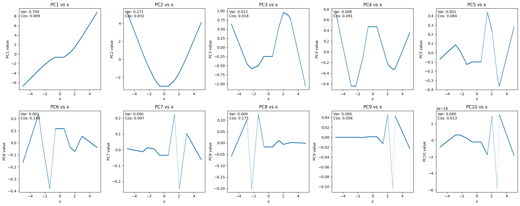
Here is Sonnet 3.6's 1-shot output (colab) and plot below. I asked for PCA for simplicity.

Looking at the PCs vs x, PC2 is kinda close to giving you x^2, but indeed this is not an especially helpful interpretation of the network.

Good post!
This was also my hypothesis when I first looked at the table. However, I think this is mostly an illusion. The sample means for rare tokens will have very high standard errors and so it is the case that rare tokens will have both unusually high average KL gap and unusually negative average KL gap mostly. And indeed, the correlation between token frequency and KL gap is approximately 0.
Yes this a good consideration. I think
- KL as a metric makes a good tradeoff here by mostly ignoring changes to tokens the original model treated as low probability (as opposed to measuring something more cursed like log prob L2 distance) and so I think captures the more interesting differences.
- This motivates having good baselines to determine what this noise floor should be.
This is a great comment! The basic argument makes sense to me, though based on how much variability there is in this plot, I think the story is more complicated. Specifically, I think your theory predicts that the SAE reconstructed KL should always be out on the tail, and these random perturbations should have low variance in their effect on KL.
I will do some follow up experiments to test different versions of this story.
Right, I suppose there could be two reasons scale finetuning works
- The L1 penalty reduces the norm of the reconstruction, but does so proportionally across all active features so a ~uniform boost in scale can mostly fix the reconstruction
- Due to activation magnitude or frequency or something else, features are inconsistently suppressed and therefore need to be scaled in the correct proportion.
The SAE-norm patch baseline tests (1) but based on your results, the scale factors vary within 1-2x so seems more likely your improvements come more from (2).
I don’t see your code but you could test this easily by evaluating your SAEs with this hook.
Yup! I think something like this is probably going on. I blamed this on L1 but this could also be some other learning or architectural failure (eg, not enough capacity):
Some features are dense (or groupwise dense, i.e., frequently co-occur together). Due to the L1 penalty, some of these dense features are not represented. However, for KL it ends up being better to nosily represent all the features than to accurately represent some fraction of them.
Huh I am surprised models fail this badly. That said, I think
We argue that there are certain properties of language that our current large language models (LLMs) don't learn.
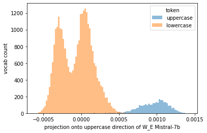
is too strong a claim based on your experiments. For instance, these models definitely have representations for uppercase letters:

In my own experiments I have found it hard to get models to answer multiple choice questions. It seems like there may be a disconnect in prompting a model to elicit information which it has in fact learned.
Here is the code to reproduce the plot if you want to look at some of your other tasks:
import numpy as np
import pandas as pd
from transformer_lens import HookedTransformer

model_name = "mistralai/Mistral-7B-Instruct-v0.1"
model = HookedTransformer.from_pretrained(
    model_name,
    device='cpu',
    torch_dtype=torch.float32,
    fold_ln=True,
    center_writing_weights=False,
    center_unembed=True,
)

def is_cap(s):
    s = s.replace('_', '')  # may need to change for other tokenizers
    return len(s) > 0 and s[0].isupper()

decoded_vocab = pd.Series({v: k for k, v in model.tokenizer.vocab.items()}).sort_index()
uppercase_labels = np.array([is_cap(s) for s in decoded_vocab.values])

W_E = model.W_E.numpy()
uppercase_dir = W_E[uppercase_labels].mean(axis=0) - W_E[~uppercase_labels].mean(axis=0)
uppercase_proj = W_E @ uppercase_dir

uc_range = (uppercase_proj.min(), uppercase_proj.max())
plt.hist(uppercase_proj[uppercase_labels], bins=100, alpha=0.5, label='uppercase', range=uc_range);
plt.hist(uppercase_proj[~uppercase_labels], bins=100, alpha=0.5, label='lowercase', range=uc_range);
plt.legend(title='token')
plt.ylabel('vocab count')
plt.xlabel('projection onto uppercase direction of W_E Mistral-7b')And SORA too: https://openai.com/sora
This is further evidence that there's no single layer at which individual outputs are learned, instead they're smoothly spread across the full set of available layers.
I don't think this simple experiment is by any means decisive, but to me it makes it more likely that features in real models are in large part refined iteratively layer-by-layer, with (more speculatively) the intermediate parts not having any particularly natural representation.
I've also updated more and more in this direction.
I think my favorite explanation/evidence of this in general comes from Appendix C of the tuned lens paper.
This seems like a not-so-small issue for SAEs? If there are lots of half baked features in the residual stream (or feature updates/computations in the MLPs) then many of the dictionary elements have to be spent reconstructing something which is not finalized and hence are less likely to be meaningful. Are there any ideas on how to fix this?
For mechanistic interpretability research, we just released a new paper on neuron interpretability in LLMs, with a large discussion on superposition! See
Paper: https://arxiv.org/abs/2305.01610
Summary: https://twitter.com/wesg52/status/1653750337373880322
There has been some work on understanding in-context learning which suggests that models are doing literal gradient descent:
- Transformers learn in-context by gradient descent
- What learning algorithm is in-context learning? investigations with linear models
- Why Can GPT Learn In-Context? Language Models Secretly Perform Gradient Descent as Meta-Optimizers
Superposition allows the model to do a lot of things at once. Thus, if the model wants to use its space efficiently, it performs multiple steps at once or uses highly compressed heuristics even if they don’t cover all corner cases. Especially in feed-forward models, the model can’t repeatedly apply the same module. Thus, implementing a “clean” algorithm would require implementing a similar algorithm in multiple layers which seems very space inefficient.
I think the first and last sentence are inconsistent. Since superposition lets you do so much at once, you can get away with having this redundancy in every layer, especially if this capacity is dedicated to a general search process that would reduce loss across a wide variety of tasks.
When models are trained to solve small optimization tasks like Knapsack, they will not rediscover either the recursive or the dynamic programming solution
I think it depends on the problem size. If the number of layers is greater than the max weight, then I would expect the model to implement the DP algorithm (and if less, I wouldn't be surprised if it still implemented an approximate DP algorithm).
In general though, I agree that the bounded depth is what makes it hard for a transformer to implement general optimization procedures.
Many parts of west Texas are also suitable for wind power which could potentially be interspersed within a large solar array. Increasing the power density of the land might make it cost effective to develop high energy industries in the area or justify the cost of additional infrastructure.
One website dedicated to this: https://aisafetyideas.com/
You could hope for more even for a random non-convex optimization problem if you can set up a tight relaxation. E.g. this paper gives you optimality bounds via a semidefinite relaxation, though I am not sure if it would scale to the size of problems relevant here.
Would love to see more in this line of work.
We then can optimize the rotation matrix and its inverse so that local changes in the rotated activation matrix have local effects on the outputted activations.
Could you explain how you are formulating/solving this optimization problem in more detail?
Could you describe your inner thought loop when conducting these sorts of mechanistic analyses? I.e., What Are You Tracking In Your Head?
Indeed, it does seem possible to figure out where simple factual information is stored in the weights of a LLM, and to distinguish between knowing whether it "knows" a fact versus it simply parroting a fact.
In addition to Google scholar, connected papers is a useful tool to quickly sort through related work and get a visual representation of a subarea.