Some additional SAE thoughts

post by Hoagy · 2024-01-13T19:31:40.089Z · LW · GW · 4 comments

Contents

  How can distributed features in an MLP work?
    Summary
    The need for non-linearity
    Basis-aligned and distributed Features
    Scaling up by sqrt(n) recovers the non-linearity
    Positive and negative feature directions
    Trading between interference and number of dimensions
  The problem of multilayer features
    The concern
    A simple experiment
  Why should we expect SAEs to work at all?
    Why would an L1 penalty even work?
    Why I think that sparse autoencoders have better priors than more complex methods in the literature for the task of finding feature vectors
None
4 comments

Thanks to Lee Sharkey for feedback on the first section and Lee Sharkey, Jake Mendel, Kaarel Hänni and others at the LISA office for conversations around this post.

This post is a collection of a few small experiments and thoughts from the last couple of months that never really turned into anything larger but have helped clarify my thinking on some SAE-related things. I've now joined the interpretability team at Anthropic but everything written here is from before that date.

How can distributed features in an MLP work?

Summary

While working on the original SAE paper, I was troubled by the following argument:

• To understand what an MLP layer is doing we need to understand how the non-linearity acts on the data, because this is where the novel computation is.
• Features as found by sparse autoencoders in the post-non-linearity of a transformer MLP seem to be very strongly distributed across neurons.
• A feature that's spread over a large number of neurons will have only a tiny effect on each individual neuron, and the neuron will be approximately linear across such a small change.
•  Therefore these distributed features can't be where the real action is, and we need to somehow incorporate the neuron basis into the way we understand features in MLPs.

I no longer believe this, most importantly because I realised that when a feature is spread across $n$ neurons, the original non-linearity can be recovered by scaling the magnitude of the input feature up by a factor of $\sqrt{n}$. The fact that it only requires scaling by $\sqrt{n}$ , rather than by $n$ which was implicit in my informal argument (when I considered the possibility of scaling up at all..) makes it feasible to use multiple highly distributed features, as long as only a small number of features are active.

Code available on GitHub.

The need for non-linearity

A multilayer model acts on input data, manipulating it into new structures at each layer. If we look at the total amount of information that is present at each successive layer, we know that the amount of information can only decline, since any information present at a higher layer is directly calculated from the lower layers, so the information must also be present in those lower layers.

However, what the model can do is to make particular functions of the data more accessible through the operation of multiple layers. In particular, the model makes rich features able to be extracted by linear probes, for example as recently seen in Language Models Represent Space and Time, and many previous works.

Linear probes are a natural test of what information is truly available, rather than hiding within the high-dimensional data manifold, as being linearly available allows subsequent neurons to condition on the presence or absence of this feature of the data.

Importantly, a linear transformation of the data cannot make new information linearly available. If we have a linear transformation $A$ that would allow us to extract information from our feature activations $x$ using a linear probe $\sigma (p\cdot Ax)$, we can remove the need for $A$ by defining a new probe $\sigma (p^{\prime }\cdot x)$ using $p^{\prime }=A^{T}p$. Therefore, if we want to make new information available in this sense, we will need to perform non-linear transformations of it, and this is where the MLP layers of a transformer come in.

Basis-aligned and distributed Features

With this need for non-linearity in mind, I want to explore how features might be constructed in a model where we move from thinking of features in an MLP as being the output of a single neuron, to being a direction that is distributed across many neurons.^[1]

For this section I will work with a 100-neuron MLP, and two potential features, one which is aligned to a single neuron and one which is spread across all 100 neurons. These will help understand some simple differences between basis-aligned and distributed features.

 A feature is defined as a direction with unit norm, so $f\in R^{100}$, $||f||=1$.

Feature 1 is simply the first neuron, $f^1=(1,0,0,...)$

Feature 2 is maximally spread across the neurons, $f^2=(0.1,0.1,0.1,...)$

Note that we're setting the $L^2$ norm to 1, (not the $L^1$ norm) and so the calculation of the feature direction is ${\sum }_i{f}_i^2=1$ so $f_i^2=0.01,f_i=0.1$.

We can interpret these as features in both in the pre- and post- non-linearity space, and look at how the features affect each other. We can look at the following relationship, where $f^i\in f^1,f^2$ is the chosen input feature and $f^o\in \{f^1,f^2\}$ is the chosen output feature, $x$ is the scalar level of input of that feature and $y$ is the scalar level of output of that feature.

$y=f^o\cdot GELU\left(x{f}^i\right)$ 

The four possible input output relationships are plotted below - before looking, I'd encourage you to think what the relationships will look like, especially between the spread input and the spread output will look like..

---

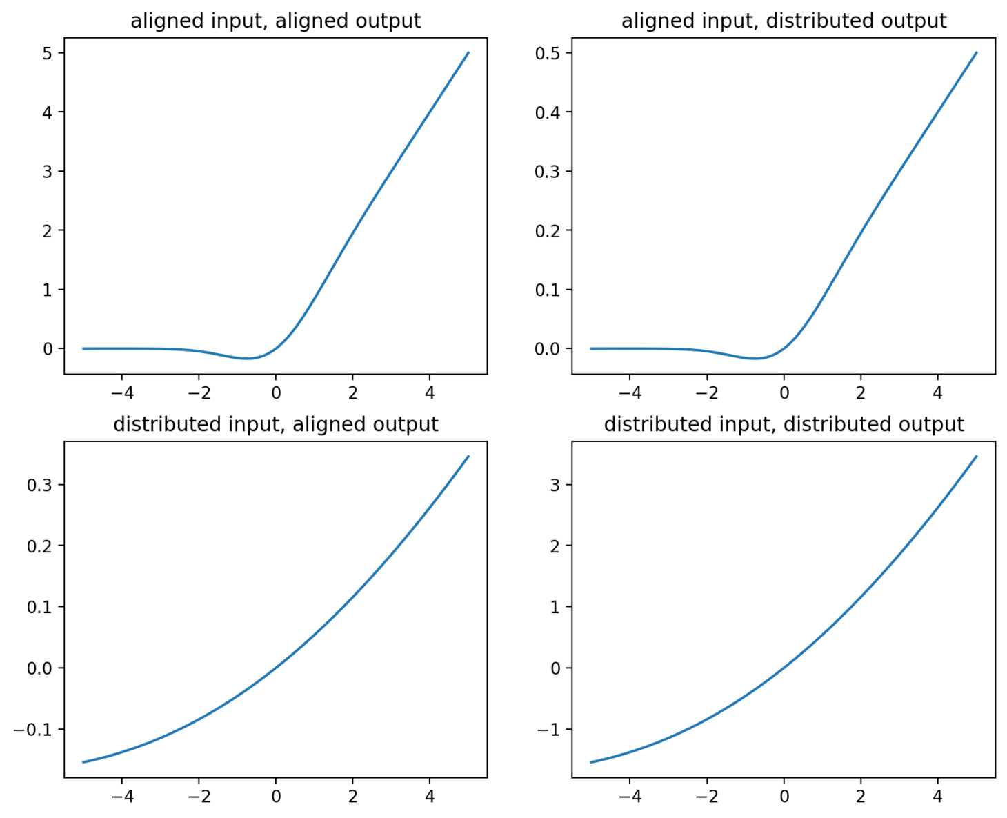
Note that the scales of each graph are different - the y-axes are rescaled to show the similarities in shape. In the top left we simply see the GELU non-linearity. In the top right, we see the same shape, but as we'd expect, the magnitude of the output is 1/10th of when using the single 

In the bottom left we see a much zoomed-in version of the non-linearity in the single-in single-out case since we're changing neuron that we care about by only 10th of the expected amount. Not only does the size of the change become small but the non-linearity is now barely noticeable.

The bottom-right is the interesting case. Importantly, although the input and output features are identical, we don't replicate the behaviour of the top-left. Instead, what we see is the behaviour of the bottom left but replicated over all 100 neurons. The scale of the output is 10x greater, since we have replaced a single (0.1 x 1) calculation with 100 x (0.1 x 0.1).

Scaling up by sqrt(n) recovers the non-linearity

The bottom-right graph is uncomfortably close to linear and wouldn't be much use as a non-linearity function. Instead, if we want to recover the same non-linearity, we need to increase the scale of variation in our input direction by $\sqrt{n}=\sqrt{1}00=10$, in which case we get the following:

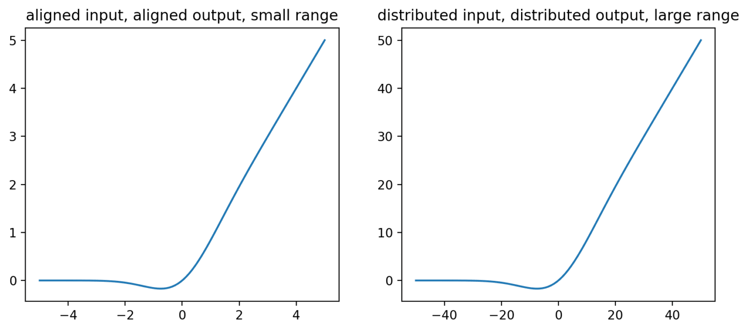
This is an example of what we mean when we say that the MLP has a preferred basis and is not invariant to rotation - in order to get the same non-linearity for a feature spread across $n$ neurons we've had to scale up our input feature by $\sqrt{n}$. Note that the scale of the output has also now increased by the same amount.

We can also somewhat see how this might generate additional robustness- if we strongly turn on another feature which is at exactly the same direction then theres simply no additional non-linearity to use, whereas here it is very likely that we be in the 'knee' of the non-linearity for lots of the neurons and therefore will get a non-linear response.

Positive and negative feature directions

Note that the above relies on all of the vector elements being positive. If we have even numbers of positive and negative elements then they cancel out and fail to produce much of a non-linearity, and if we have somewhat unbalanced combinations then we get intermediate cases with somewhat attenuated non-linearities.

Therefore we should expect our incoming feature vectors to be skewed heavily towards positive or negative components, if they are to make new information linearly available.

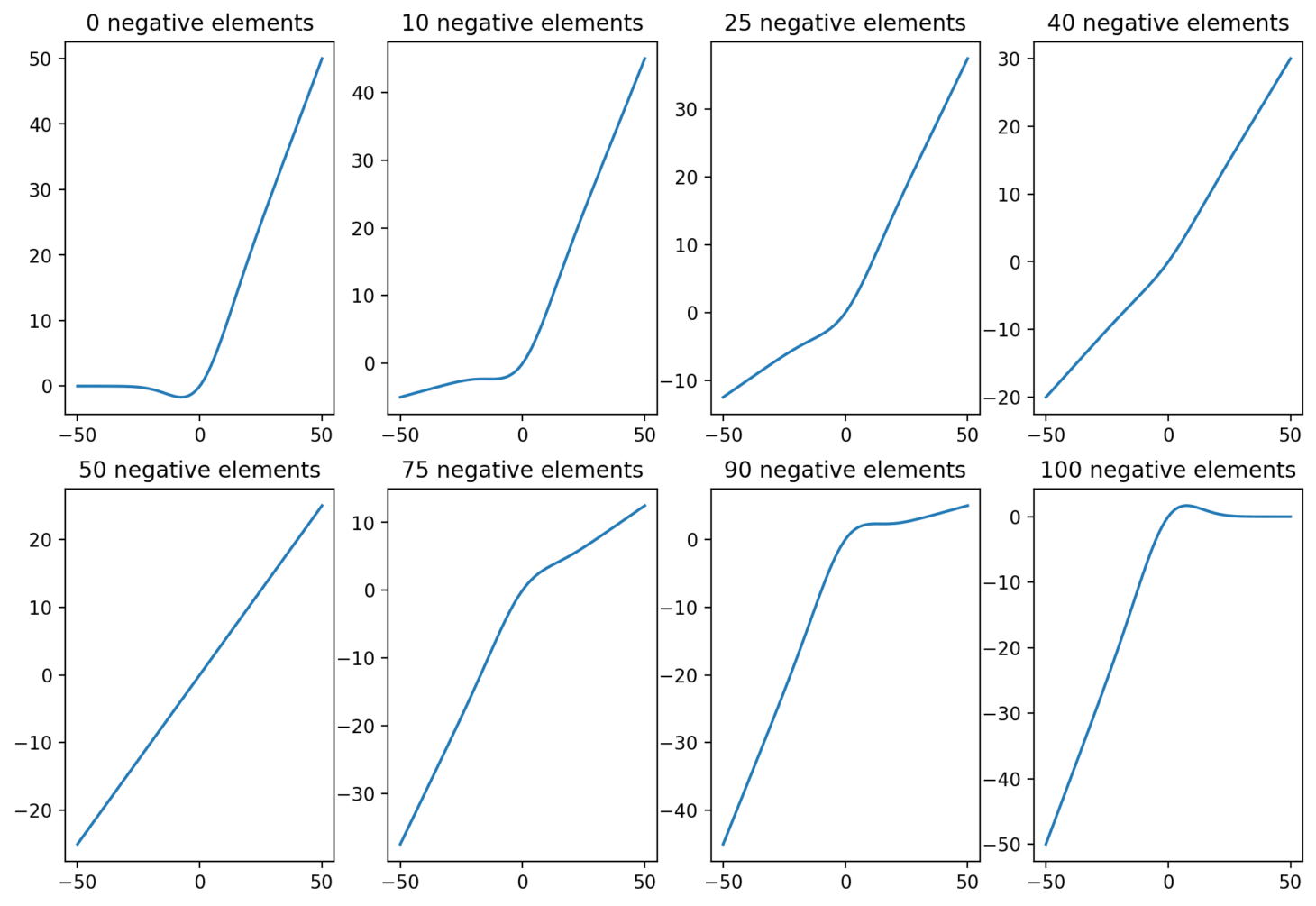
This also implies some limit to the number of possible features in the MLP. Johnson-Lindenstrauss tells us that the number of nearly-orthogonal features in a high-dimensional space is exponential in the dimension of that space, but the majority of these dimensions will have nearly balanced amount of positive and negative components and therefore will not be useful in a non-linearity as the output in this direction will be a homogeneous function of the input in that direction.

We can see how, using these distributed functions, we can still think of networks as putting the thing that they want amplified in the positive direction of neurons but doing this over many dimensions.

Trading between interference and number of dimensions

By scaling up the magnitude of our input features, we've recovered the original non-linear behaviour of the individual neurons. However, intuitively we would expect that making the magnitude of our input larger, feeding into non-linearities which have a fixed scale, should have consequences for how many features we can have active at any one time because the level of interference will be greater.

One important note of terminology (with thanks to Jake Mendel): linearity is the condition that $f(ax+by)=af\left(x\right)+b\left(y\right)$, while homogeneity is the weaker condition that $f\left(ax\right)=af\left(x\right)$. While linearity is ultimately the thing I am interested in, what I am measuring in this case is homogeneity in a particular input direction, and so I will switch to this terminology where appropriate.

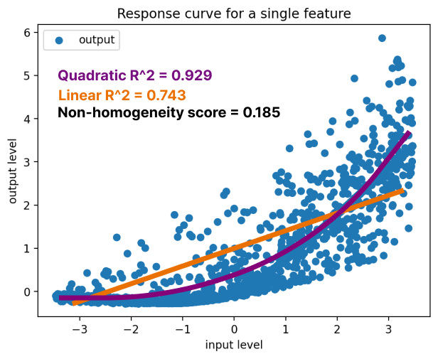
To understand whether and when this becomes an issue, I plot the input-output response curve for a particular direction. The algorithm is as follows:

• I generate a set of feature vectors, each of which is a direction in the input/output space with only a fixed number of non-zero elements, dims_per_feature
• I set a fixed number of features, n_on, other than the feature of interest, which will be on at any one time
• I select a random input feature, and generate a set of inputs to the non-linearity where the feature, and n_on other features, are all active, with a magnitude that varies evenly in -np.sqrt(dims_per_feature) < mag < np.sqrt(dims_per_feature) 
• I pass these input vectors through the non-linearity to get output vectors, and project these output vectors onto the feature of interest, to get the feature level in the output.
• I run regressions to predict the level of the chosen feature in the output, as a function of the level of the feature in the input
• I measure the degree of non-homogeneity by taking the degree of feature activation before and after the non-linearity and calculating a simple regression to predict the post-non-linearity feature values from the pre-non-linearity feature values. The first regression has just this single input parameter. The second includes a quadratic term - just the input value squared.

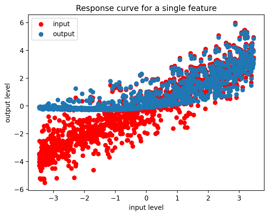
If there's significant non-homogeneity then the quadratic regression should be able to better predict the output values than the linear regression.

The output metric is the difference in $R^2$ between the quadratic and linear regressions on a test set consisting of 20% of the data being held out. This gives us a simple measure of the degree to which we see a non-homogeneous response from varying the input.

What we can then do is take a fixed width of network, here still $n=100$, and vary the number of dimensions that each feature is spread across. We can set a threshold for the 'level of non-homogeneity' and see how many features can be active at any one time, before we consider the relationship to be roughly homogeneous. Here I arbitrarily set this threshold to 0.1. 

At the same time we can plot, for a given number of dimensions per feature, how many nearly orthogonal features we can have, using as a proxy for this the mean max cosine similarity (MMCS) of a random set of feature vectors. We take the number of nearly orthogonal features to be the point at which the MMCS gets above a certain threshold, here chosen as 0.3. This is certainly an underestimate as the network could arrange the features to be more precisely orthogonal than a random subset but it gives a rough idea.

All this is done so that we can see that there is in fact a somewhat sensible seeming tradeoff where by increasing the number of dimensions per feature, we allow ourselves more almost-orthogonal feature vectors, at the cost of being able to have few active features before interference swamps the non-linearity and removes our ability to do interesting work with the layer (at least by this simply non-homogeneity meas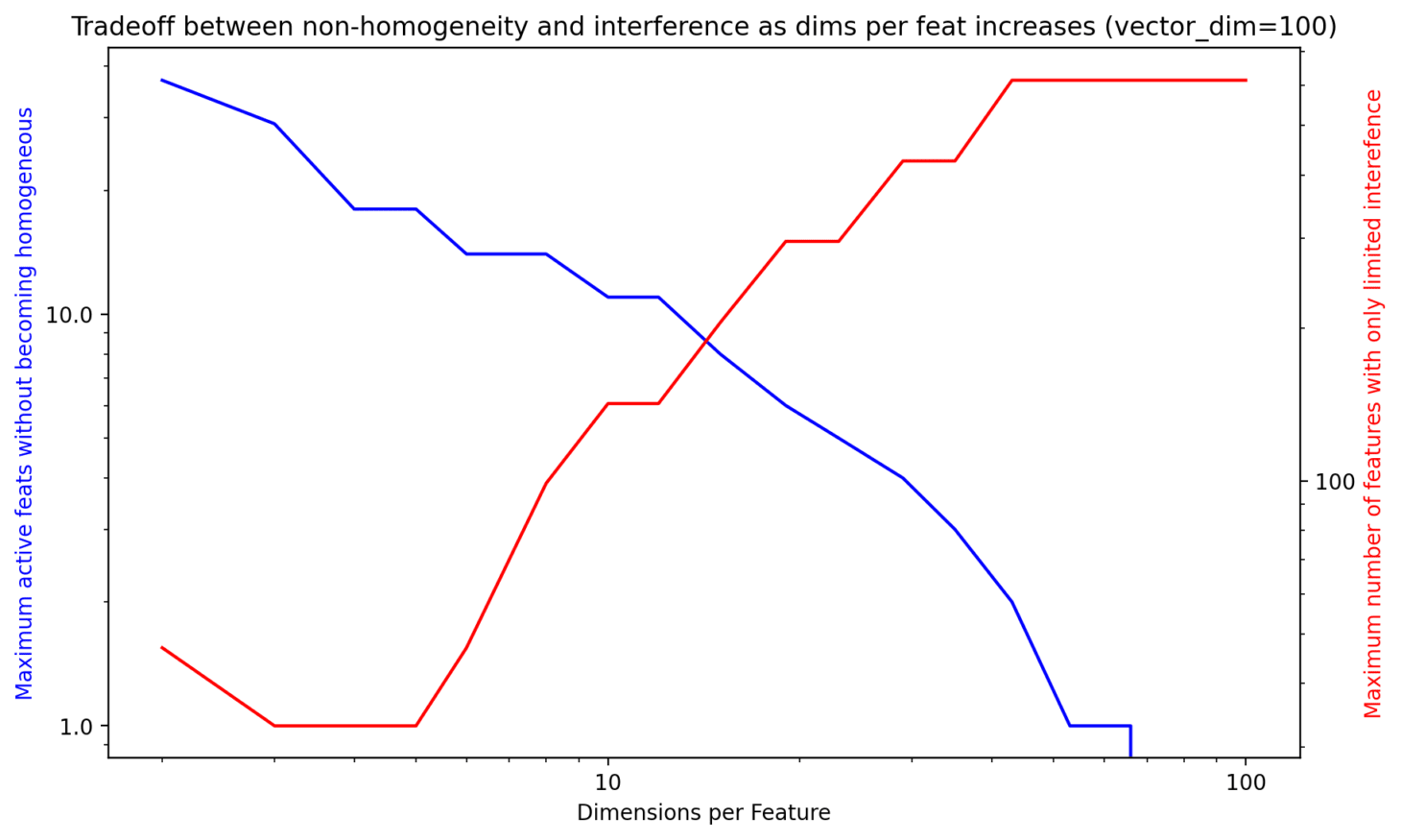ure).

This closely mirrors the conclusions reached in much more detailed fashion in the Toy Models of Superposition paper which explores the role of superposition in an idealised residual stream and gives some theoretical backing to how it's possible to find distributed features in an MLP.

The problem of multilayer features

The concern

One way in which sparse autoencoders could fail to deliver on their promise is that we have something like 'completed features' and 'in progress features'. For example a feature is to be read at layer 20, while the prerequisite elements are in place at layer 10 but, rather than the feature being learned within a single layer in (10, 20) the model finds it advantageous to build the feature incrementally, perhaps because this increases the number of features that can be built concurrently, or perhaps just because it's not costly and there are many more distributed than non-distributed ways to create a feature.

A motivating example here, one of many, is the Gurnee and Tegmark (2023) paper which probed for longitude and latitude representations across the layers of Llama models.

If we were to look at this through the lens of a sparse autoencoder - or any other basis-finding approach - we might find a latitude direction once it's 'fully built' - but what would we expect to find as those layers are being built up?

 

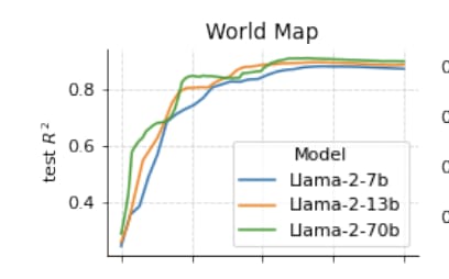
There's a few different experiments one might do to look at these questions - here I've just run one of the simplest potential tests to see whether there was in fact a tendency to concentrate the learning of a particular connection into a single layer.

A simple experiment

The set up is a simple model of an MLP-only transformer, consisting of a series of hidden layers with residual connections at each layer. The input is a pair of one-hot vectors, meaning that if the vector dimension is 500, the input will be a 1000-dimensional vector with one active dimension in the first 500, and one active dimension in the second 500. These are projected to the hidden dimension which is the same as the output width by a learned vector, and then there is a series of MLP layers with recurrent connections, each with the same width.

First we can check the overall loss after each layer, evaluating the loss on the output after each layer. What we find is that there's close to a linear reduction, at least in the later layers, showing that the model is iteratively making the residual stream closer to the desired output.

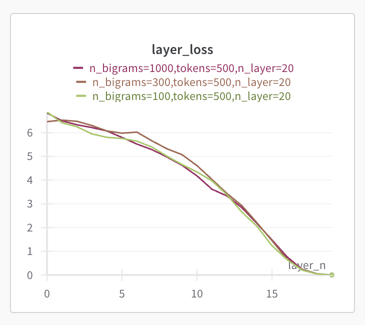
You can imagine two opposite ways that the model would calculate this - at one end, each layer would compute the correct output for a particular subset of the input. At the opposite end of this spectrum, the input would be continually transformed until the answer for each of the datapoints was finally made correct in the very final layer, with each layer doing some degree of intermediate processing.

For a simple test of which of these two pictures was closer to the truth, I then took the logit lens output after each layer for individual datapoints, and taking just a few randomly selected datapoints I got graphs like the following:

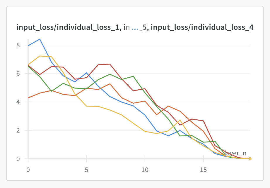
This already gives us the information that we need, but just in case these are outliers, we can take some threshold of loss as a proxy for whether the output is correctly learned by a certain layer and then plot the fraction of the datapoints that are learned, and we get the following (threshold=0.1):

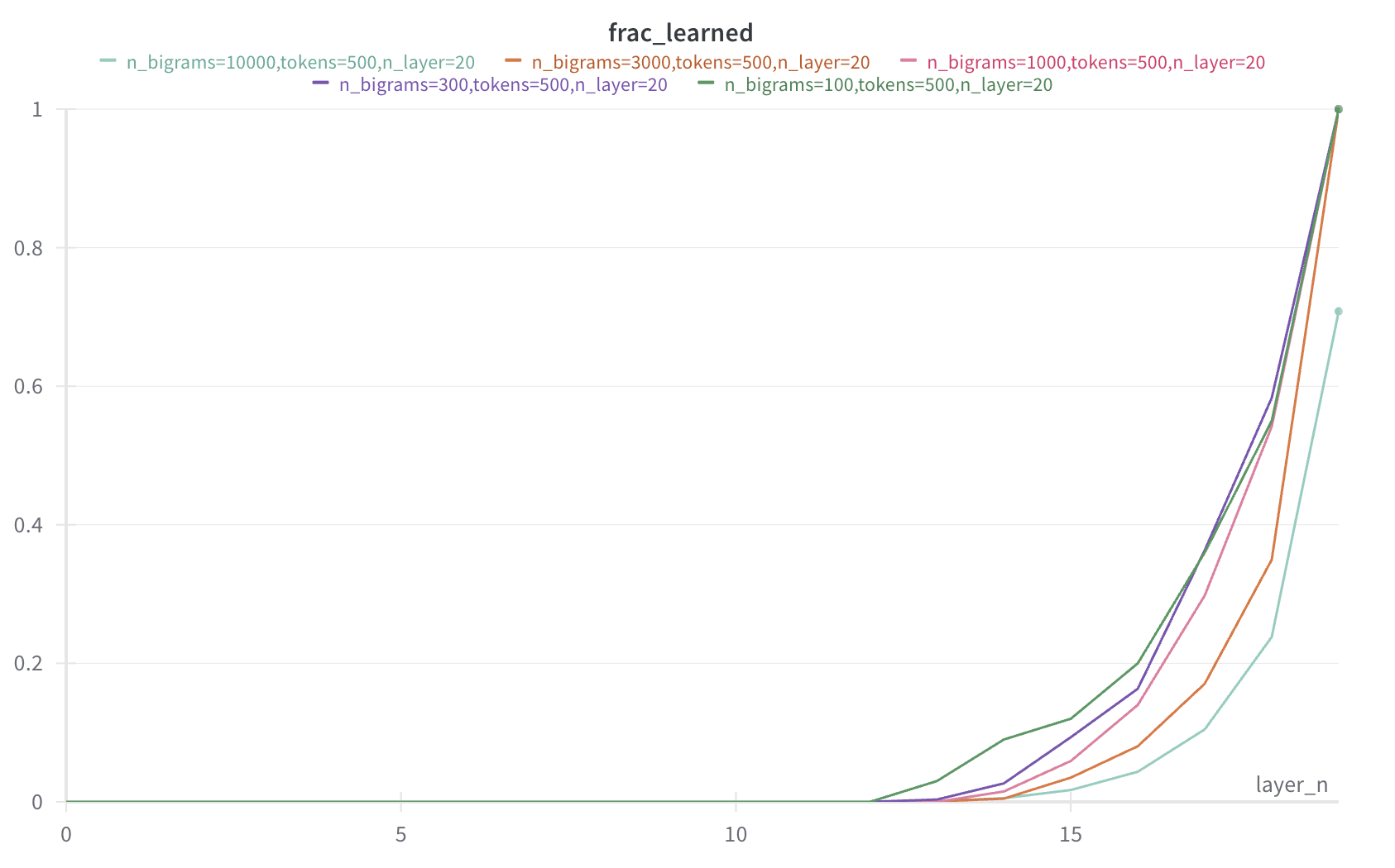
Again we see what was already evident in the first graph - that the different datapoints only become fully learned right near the end - though there is some degree of variation. More interestingly, where the number of unique datapoints is larger, the fraction of datapoints successfully meeting the threshold is higher, even when they can all be learned eventually. This is evidence that calculating a layer in a distributed manner with respect to the layers is a more efficient solution for the model than to calculate them in separate layers.

I also had a look to see whether, for individual features, there was still something like a 'decisive' layer when it came to deciding which output. I looked at, for individual datapoints, the norm of the gradient of each layer's weight matrix, when the gradient is calculated with respect to the correct output, rather than the loss.

optimizer.zero_grad()
output = model(inputs[i])
correct_output = output[targets[i]] # getting the target for a single datapoint
correct_output.backward()
for layer_n in range(n_hidden_layers):
    wandb.log(
        {
        f"grads/layer_grad_{i}_output": torch.norm(
                model.hidden_layers[layer_n].weight.grad
            ),
            "layer_n": layer_n,
        }
    )

Again we don't see any particular peak:

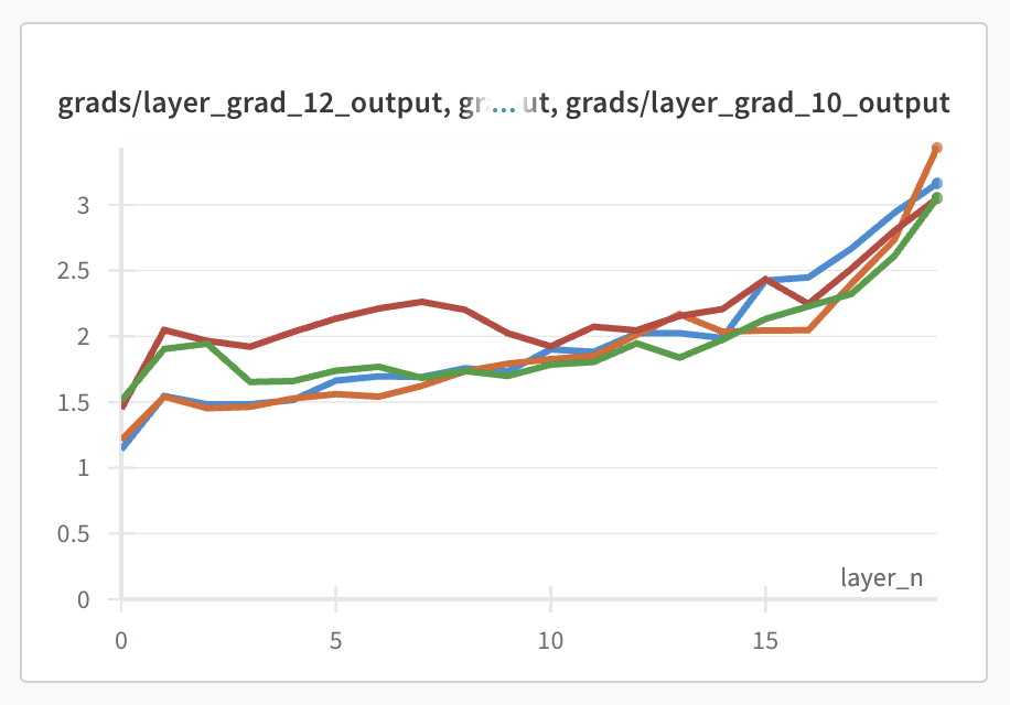
This is further evidence that there's no single layer at which individual outputs are learned, instead they're smoothly spread across the full set of available layers.

I don't think this simple experiment is by any means decisive, but to me it makes it more likely that features in real models are in large part refined iteratively layer-by-layer, with (more speculatively) the intermediate parts not having any particularly natural representation. This is not to say there wouldn't be hierarchical features, but if the depth of the hierarchy is much smaller than the number of layers, then you wouldnt expect to be able to interpret the MLP layers of a model in isolation.

As an aside, I'd be really interested to see people doing mechanistic interpretability on these sort of simple algorithmic tasks to expand the library of how models do these kinds of super basic tasks.

Another things that one could so is to train an SAE for all layers of the model that they found their longitude and latitude vector on, and check to what extent there's a learned dimension which is similar to the one which is found in the Gurnee paper.

Why should we expect SAEs to work at all?

Why would an L1 penalty even work?

While I knew that empirically that L1 losses were a good differentiable substitute for an L0 penalty, I had incorrect pictures in my head for why this was the case for a long time.

A basic question about the L1 penalty asks 'wait, but if we have vector X with magnitude 5.0, and basis vectors $Y_1,Y_2,...,Y_n$ which we could build with either $5Y_1$ or $Y_2+Y_3+Y_4+Y_5+Y_6$, then (ignoring coefficient) the L1 loss would be 5 in both cases, so it seems like this doesn't actually incentivise sparsity?'

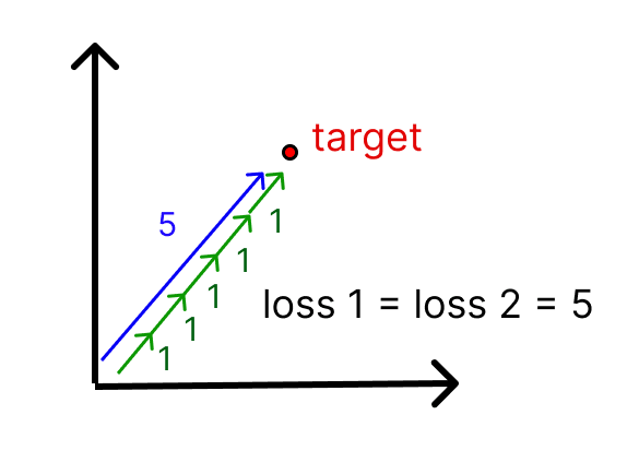
This objection that L1 penalties fail to incentivise sparsity is correct when we have multiple basis vectors which point in equally similar directions, but this is a special case that only occurs when two dictionary elements point in the same direction. It only requires a tiny difference in the degree of similarity to break the equality and favour the more sparse solution. If we have a 2D space, and three directions where each pair is linearly independent, then to choose the most efficient way, we'll pick a 1 feature solution when possible, and a 2 feature solution, with greater weight on the closer solution, when there's no 1D solution. 

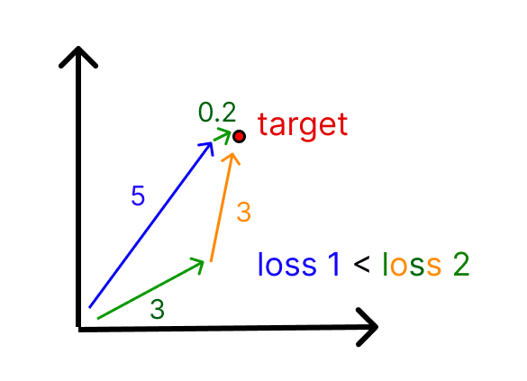
To understand it another way, assuming that we reconstruct our input vector perfectly, the L1 loss will be inversely proportional to the average cosine similarity of the features used to reconstruct the features, weighted by how much each feature is active, and so it pushes towards using the most cosine-similar features as much as possible.

Of course, the sparse autoencoder isn't able to do the optimisation to find the best available solution but it should approximate this process as well as it can with its simple linear encoder and thus should still have the same approximate properties.

At the same time, we should not expect the sparse autoencoder to learn two highly similar directions in the first place, because having two vectors in the same direction will give no benefit when they're both used, while missing out on the opportunity to incorporate some other, useful direction into the dictionary.

Why I think that sparse autoencoders have better priors than more complex methods in the literature for the task of finding feature vectors

Sparse autoencoders are a very simplistic approach to the more general sparse coding problem. In the general setting we have a dictionary of features, and we want to calculate which small subset of the features went into creating each example, and to which degree (the coefficients, aka feature vector). 

In standard approaches to sparse coding are freely optimized, with no closed-form relationship between input vector and feature levels. This freedom is helpful in many signal processing cases. For example, an image is a low dimensional representation of a much more detailed reality. There's no particular reason that two very different configurations of reality could look almost identical in a photo, and therefore it might take a lot of careful detective work to understand which of two possible configurations did in fact produce the photo.

The situation for neural networks is very different, because if two radically different sets of features resulted in the same residual stream then the network itself will struggle to separate the two. Instead, the network wants the information to be easy to read off using the tools it has, which are largely linear maps ($W_{in},W_Q$, $W_V$, $W_K$). 

Aidan Ewart tried using a multilayer encoder rather than the single Linear+ReLU of the standard SAE. He found it difficult to match the performance and the resulting features didn't seem as interpretable. I think this is because it removes the benefit of having a prior on how to read features which is close to how the network will read them.

This doesn't mean that current SAEs are optimal though. There's an issue where the encoder struggles to have sufficient power to correctly predict the magnitude of the output when there are features with non-zero cosine similarity. For example, if you have features (1, 0) and ($1/\sqrt{2}$, $1/\sqrt{2}$), and the correct bias is 0, it struggles to recreate the vector (2, 1) - it wants to reconstruct it with a magnitude of $\sqrt{2^2+{\frac{3\sqrt{2}}{2}}^2}=\sqrt{8.5}$ rather than $\sqrt{5}$.

This is especially a problem for autoencoders where the weights are tied, but even an untied autoencoder only has a limited amount of flexibility.

To make improvements, we should therefore think about how to make it easier for the SAE to reconstruct the output when it has learned the correct features, while still retaining the helpful linear prior over features (or a better prior if we can understand networks better).

1. ^{^}

   Note on features - I don't think that it's true that networks are composed of a fixed number of discrete features, instead I think it's a discrete approximation to a continuous reality that I've found helpful for how to think about model internals but probably has serious limitations.

4 comments

Comments sorted by top scores.