Analysing Adversarial Attacks with Linear Probing
post by Yoann Poupart, Imene Kerboua (imenelydiaker), Clement Neo (clement-neo), Jason Hoelscher-Obermaier (jas-ho) · 2024-06-17T14:16:33.832Z · LW · GW · 0 commentsContents
  TL;DR
  Introduction
    Motivation
    Hypotheses to Test
    Post Navigation
  Background
    Adversarial Attacks
    Linear Probing
  Experiments
    Models Setup
      Dataset Creation
      Classifier Training
      Probe Training
      Sanity Checks
    Analysing Adversarial Attacks with Linear Probing
      Goal
      Setup
      Lemon -> Tomato
      Lemon -> Tomato (Layer 6 & Layer 0)
      Lemon -> Banana
      Tomato -> Lemon
    Concept Probability Through Layers: Naive Detection
  Limitations
      Interpretability Illusion
      You Need Concept in Advance
      Introduced Biases
      Truly Bugs Attacks
  Perspectives
      What’s next?
      Multimodal Settings
      Representation Engineering
  Related Work
      Analysing Adversarial Attacks
      Adversarial Attacks on Latent Representation
      Universal Adversarial Attacks (UAPs)
      Visualising Adversarial Attacks
  Conclusion
  Appendix
    Dataset description
None
No comments
This work was produced as part of the Apart Fellowship. @Yoann Poupart [AF · GW] and @Imene Kerboua [LW · GW] led the project; @Clement Neo [AF · GW] and @Jason Hoelscher-Obermaier [AF · GW] provided mentorship, feedback and project guidance.
Here, we present a qualitative analysis of our preliminary results. We are at the very beginning of our experiments, so any setup change, experiment advice, or idea is welcomed. We also welcome any relevant paper that we could have missed. For a better introduction to interpreting adversarial attacks, we recommend reading scasper [LW · GW]’s post: EIS IX: Interpretability and Adversaries [AF · GW].
Code available on GitHub (still drafty).
TL;DR
- Basic adversarial attacks produce humanly indistinguishable examples for the human eye.
- In order to explore the features vs bugs view of adversarial attacks, we trained linear probes on a classifier’s activations (we used CLIP-based models for further multimodal work). The goal is that training linear probes to detect basic concepts can help analyse and detect adversarial attacks.
- As the concepts studied are simple (e.g. color), they can be probed from every layer of the model.
- We show that concept probes are indeed modified by the adversarial attack, but only on the later layers.
- Hence, we can naively detect adversarial attacks by observing the disagreement between early layers’ probes and later layers’ probes.
Introduction
Motivation
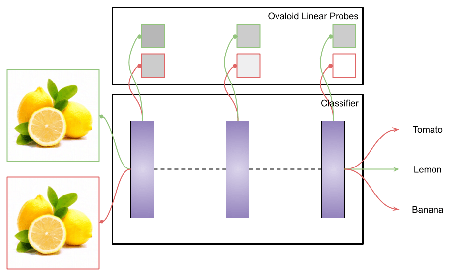
Adversarial samples are a concerning failure mode of deep learning models. It has been shown that by optimising an input, e.g. an image, the output of the targeted model can be shifted at the attacker’s will. This failure mode appears repeatedly in different domains like image classification, text encoders, and more recently on multimodal models enabling arbitrary outputs or jailbreaking.
Hypotheses to Test
This work was partly inspired by the feature vs bug world hypothesis. In our particular context this would imply that adversarial attacks might be caused by meaningful feature directions being activated (feature world) or by high-frequency directions overfitted by the model (bug world). The hypotheses we would like to test are thus the following:
- The adversariality doesn't change the features. Nakkiran et al. found truly adversarial samples that are "bugs", while Ilyas et al. seem to indicate that adversarial attacks find features.
- The different optimisation schemes don't produce the same categories of adversarial samples (features vs bugs). Some might be more robust, e.g. w.r.t. the representation induced.
Post Navigation
First, we briefly present the background we used for adversarial attacks and linear probing. Then we showcase experiments, presenting our setup, to understand the impact of adversarial attacks on linear probes and see if we can detect it naively. Finally, we present the limitations and perspectives of our work before concluding.
Background
Adversarial Attacks
For our experiment, we'll begin with the most basic and well-known adversarial attack, the Fast Gradient Sign Method (FGSM). This intuitive method takes advantage of the classifier differentiability to optimise the adversary goal (misclassification) using a gradient descent. It can be described as:
With the original image and label, the adversarial example and the perturbation amplitude. This simple method can be derived in an iterative form:
and seen as projected gradient descent, with the projection ensuring that . In our experiments .
Linear Probing
Linear probing is a simple idea where you train a linear model (probe) to predict a concept from the internals of the interpreted target model. The prediction performances are then attributed to the knowledge contained in the target model's latent representation rather than to the simple linear probe. Here, we are mostly interested in binary concepts, e.g. features presence/absence or adversarial/non-adversarial, and the optimisation can be formulated as minimising the following loss:
where in our experiments is a logistic regression using the penalty.
Experiments
Models Setup
Dataset Creation
In order to explore image concepts we first focused on a small category of images, fruits and vegetables, before choosing easy concepts like shapes and colours. We proceeded as follow:
- We curated a dataset originating from Kaggle, making sure to have proper train and test splits. We also have spotted some misclassified images.
- We then labelled (not totally finished) the presence of concepts on these images to create our concepts dataset.
- See more details in appendix.
- We trained different classifiers on this dataset, all from the CLIP vision encoder.
- We didn’t use augmentation tricks as all our classifiers already reached pretty good accuracies.
- We first created an activation dataset using the CLIP’s vision encoder. We used the residual stream activations as we are interested in full representation rather than head behaviour.
- We subsequently trained our probes on these activations.
Classifier Training
Probe Training
Sanity Checks
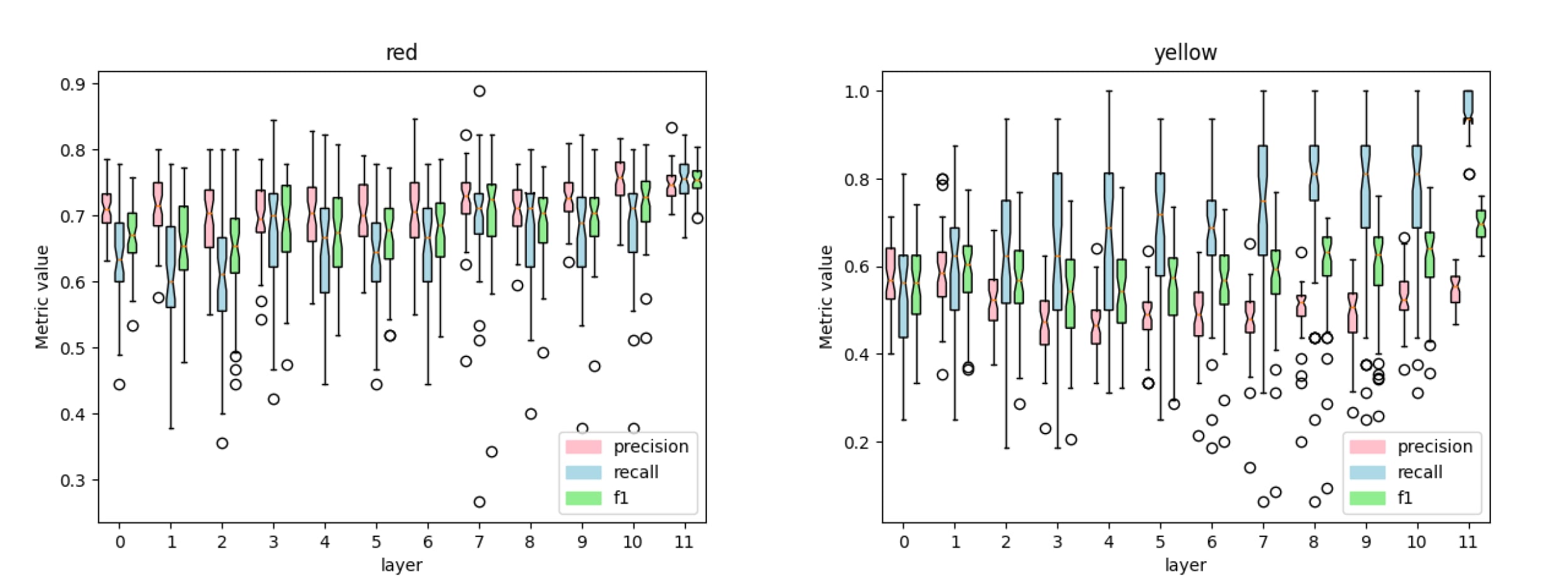
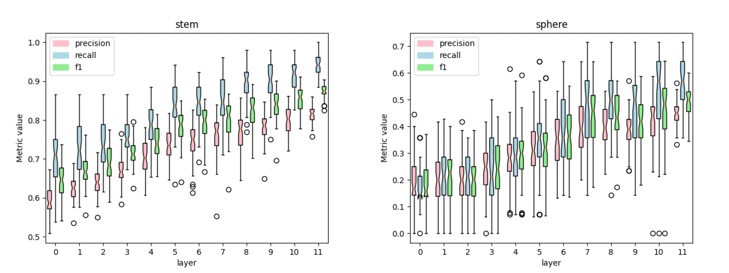
The goal is to validate that probes are detecting the concepts and not something else that is related to the class (we are not yet totally confident about our probes, more in the limitations).
- Each layer and each concept has a dedicated linear probe.
- We plot precision, recall and f1 scores for some of the trained probes, such as the one for the colour “red”, “yellow”, “stem” and “sphere”.
- Noticeably the dynamics of concepts seem different. Certain concepts like “green” are present in every layer while concepts like “sphere” seem to appear in later layers.
Analysing Adversarial Attacks with Linear Probing
Goal
See what kind of features (if any) adversarial attacks find. Increase of the probe's accuracy on non-related features w.r.t. the input sample but related to the target sample.
Setup
- Model: ViT (CLIP)
- Niche image dataset ( fruits and vegetables)
- Get or train a classifier based on CLIP (frozen)
- Label concepts in this dataset, e.g. shape/colour/category/background
- Probe before and during the iterative FGSM and see if the probe activation changes
Lemon -> Tomato
For this experiment, we show that given an input image of a lemon, it requires a few steps of adversarial perturbation for the model to output the desired target, tomato in our case (see figures 4-6).
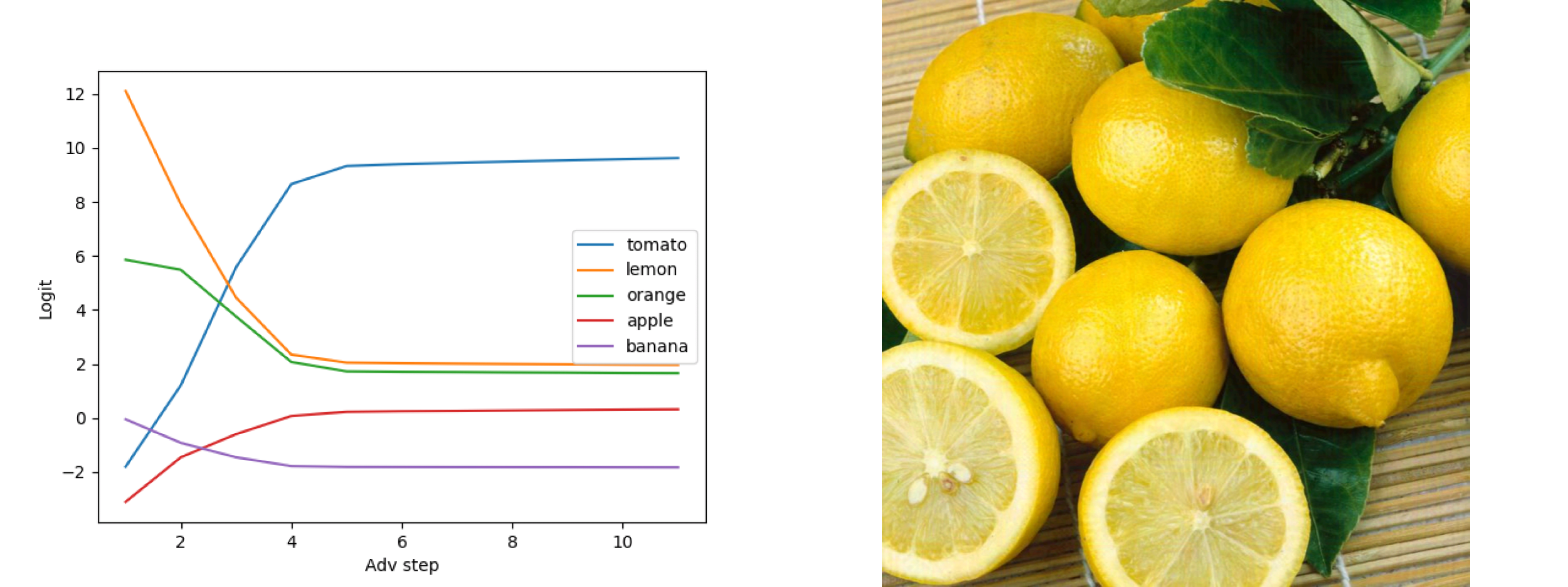

We compare the appearance of two concepts “ovaloid” and “sphere” in the last layer of the vision encoder, which are the shapes of the lemon and the tomato respectively. It appears in Figure 7 that the concept “ovaloid” characterising the lemon disappears gradually with the increase of the adversarial steps, while the “sphere” concept marking the tomato starts to appear (see Figure 8).

Lemon -> Tomato (Layer 6 & Layer 0)
We noted that the concept “sphere” which characterises a tomato, does not appear and remains unchanged in the first layers of the encoder (see Figure 9 and 10 for layers 0 and 6 respectively) despite the adversarial steps.


Lemon -> Banana
We focus our interest in a concept that characterises both a lemon and a banana, the colour “yellow”. The adversarial attack does not change the representation of this concept through the layers and the adversarial steps (see Figure 11, Figure 12 and Figure 13).


Tomato -> Lemon

Concept Probability Through Layers: Naive Detection
This section contains early-stage claims not fully backed, thus we would love hearing feedback on this methodology.
We spotted interesting concept activation patterns through layers, and we believe they could help detect adversarial attacks once formalised. We spotted two patterns:
- “genesis out of thin air” a concept going from 0 in L0 to 1 in L11. Indicating a concept being artificially activated.
- “Appear and disappear” a concept going from low in L0 to high in middle layers and the low again in L11. Indicating a concept being artificially suppressed.
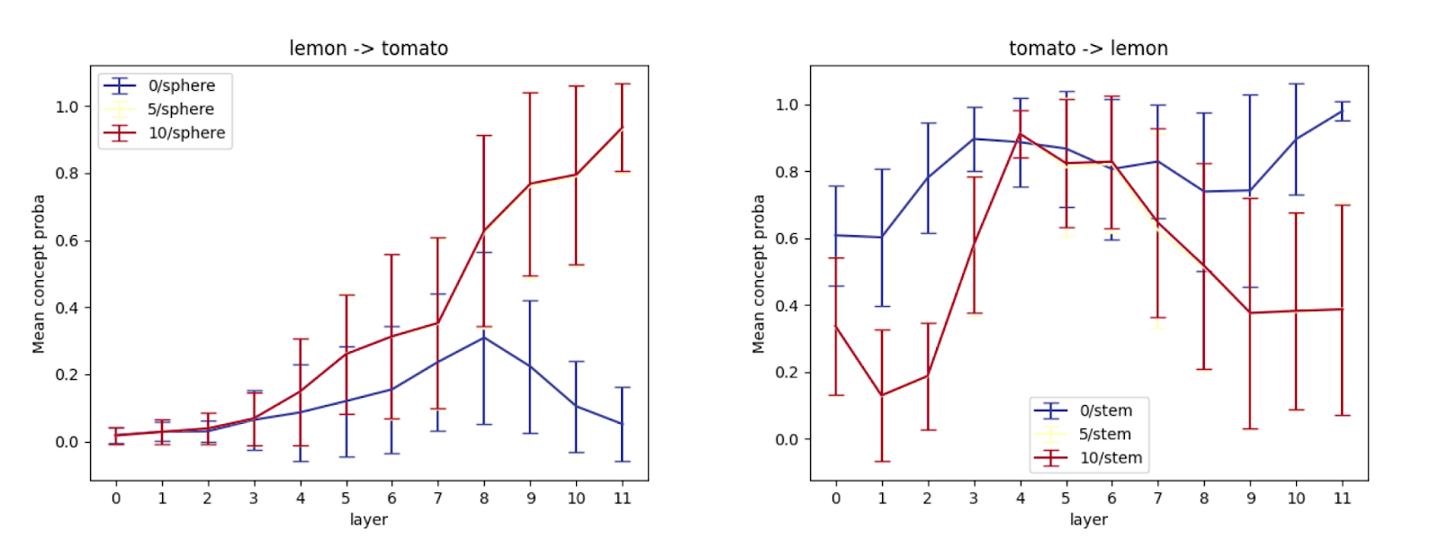
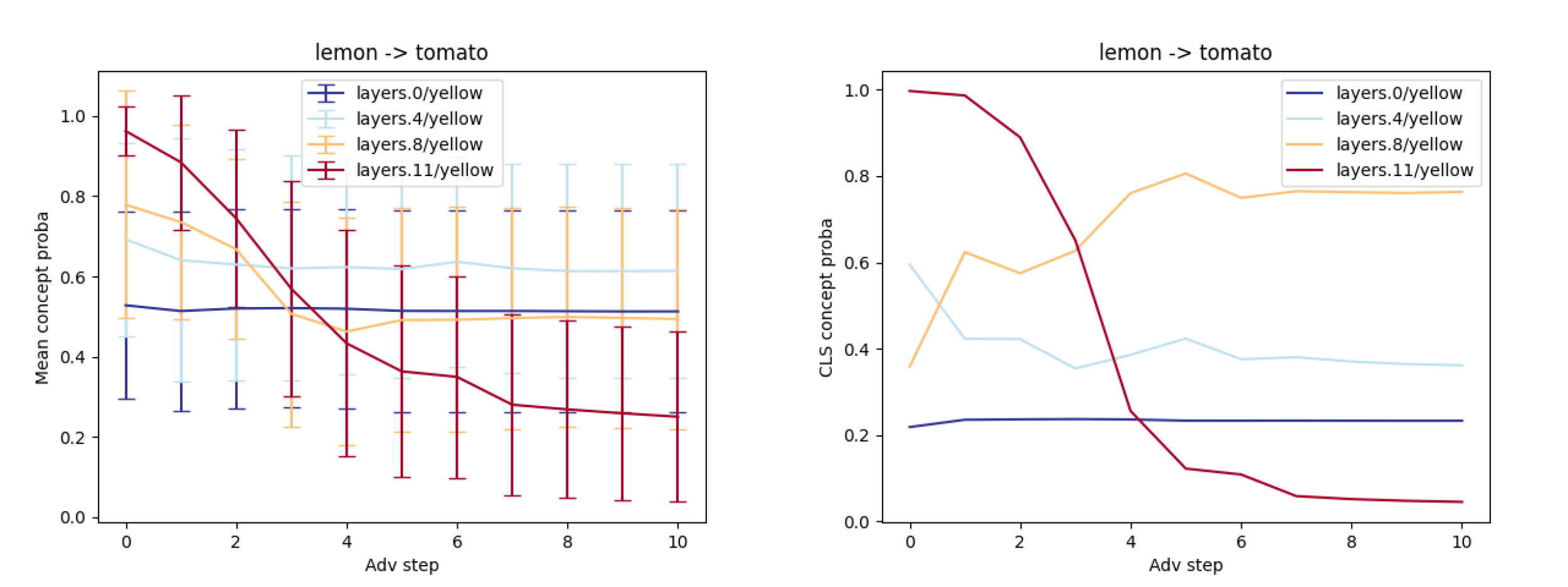
Looking at the concept curve (e.g. on the CLS in Figure 14) we see that there is a transition mostly on the last layer. This could indicate that our adversarial attacks mostly target later layers and thus could be detected spotting incoherent patterns like the probability in Figure 14 (L0: 02 -> L4: 0.35 -> L8: 0.8 -> L10: 0.0).
Intuitively this would only be fair for simple concepts that are in the early layers.
We present what we are excited to (see) tackle next in the perspectives section.
Limitations
Interpretability Illusion
Interpretability is known to have illusion issues and linear probing doesn’t make an exception. We are not totally confident that our probes do measure their associated concept. In this respect we aim to further improve and refine our dataset.
- The appearance of concepts like “sphere” in later layers might be a labelling artifact.
- We tried more robust probes but it didn’t improve the sanity checks.
- We tried only training on early layers and evaluating on all
- We tried simultaneously training on all layers
You Need Concept in Advance
- Here, without the labelled concepts, analysing the adversarial attack is impossible.
- While image classification is easy to conceptualise, multimodal settings might be more challenging. Adversarial attacks based on a text decoder might be much harder to detect.
Introduced Biases
We trained one probe per concept and per layer (on all visual tokens). Our intuition is that information is mixed by the cross-attention mechanism and similarly represented across tokens for such simple concepts.
Truly Bugs Attacks
We are not tackling some adversarial attacks that have been labelled as truly bugs. We are interested in testing our method on it as this could remain a potential threat.
Perspectives
We now describe what we are excited to test next and present possible framing of this study for future work.
What’s next?
First, we want to make sure that we are training the correct probes. Some proxies are mixed with concepts, e.g. pulp is mostly equivalent to orange + lemon. For that, we are thinking of ways to augment our labelled dataset using basic CV tricks.
We are moving to automated labelling using GPT4V, while keeping a human in the loop overseeing the labels produced. And we are also thinking about creating concept segmentation maps as the concepts localisation might be relevant (c.f. the heatmaps above).
In the longer term view, we are also willing to explore the following tweaks:
- Exploring the impact of changing the adversarial loss, e.g. without using a classifier.
- Using different classifiers, e.g. more robust classifiers.
- Explore universal adversarial attacks and non-transferable adversarial attacks.
- The same detection method could be used but for image adversarial attacks based on a text decoder.
- Compare the impact of adversarial attacks on the concepts in the text decoder and image encoder.
- Using the probe directions to create adversarial attacks.
- Using adversarial attacks to create steering vectors
Multimodal Settings
- The same detection method could be used but for image adversarial attacks based on a text decoder.
- Compare the impact of adversarial attacks on the concepts in the text decoder and image encoder.
Representation Engineering
- Using the probe directions to create adversarial attacks.
- Using adversarial attacks to create steering vectors
Related Work
Analysing Adversarial Attacks
- Dection based on explainable reinforcement learning
- Using mutual information between the origin class and the target class
- Defence via concept extraction by segmentation
- Feature robustness analysis of adversarial attacks
Adversarial Attacks on Latent Representation
- Steer the last feature layer using a target decoder
- Attack based on inner layers for increasing transferability
Universal Adversarial Attacks (UAPs)
- Analysis of generaling properties of UAPs in the continuity of Ilyas et al.
- Universal bug features
- Using distributional properties to create UAPs
- A survey on adversarial attacks
Visualising Adversarial Attacks
- Feature visualisation of adversarial attacks (features based on neuron activation maximisation)
- Visualising neuron pathways of adversarial attacks
- Visualisation of neuron vulnerability
Conclusion
Our method doesn’t guarantee that we’ll be able to detect any adversarial attacks but showcases that some mechanistic measures can be sanity safeguards. These linear probes are not costly to train nor to use during inference and can help detect adversarial attacks and possibly other kinds of anomalies.
Appendix
Dataset description
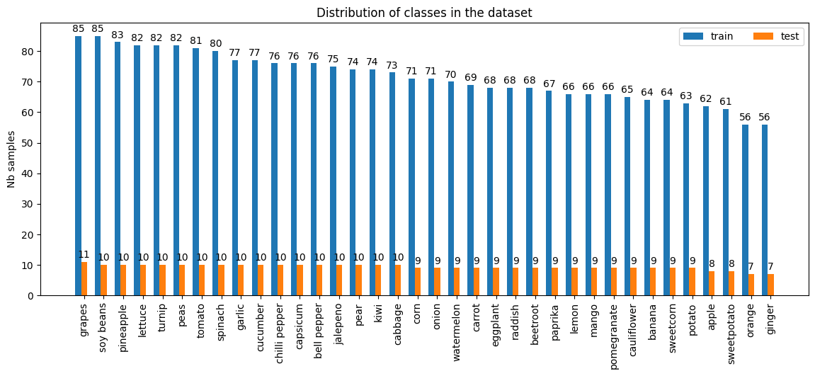
We collected a dataset of fruits and vegetables image classification from Kaggle (insert link). The dataset was cleaned and manually labelled by experts. The preprocessing included a deduplication step to remove duplicate images, and a filtering of images that were present in both the train and test sets, which encouraged data leakage.
For the annotation process, there were 2 annotators who labelled each image with the concepts that appear on it, each image is associated with at least 1 concept. An additional step was required to resolve annotation conflicts and correct the concepts.
After preprocessing, the train set contains over 2579 samples and the test set over 336 samples with 36 classes each; the class distributions over sets are shown in Figure 17.
The chosen concepts concern the colour, shape and background of the images. Figure 18 shows the distribution of concepts over the whole dataset.
0 comments
Comments sorted by top scores.