How To Do Patching Fast

post by Joseph Miller (Josephm) · 2024-05-11T20:13:52.424Z · LW · GW · 6 comments

Contents

  What is activation patching?
    Node Patching
    Edge Patching
    Path Patching
  Fast Edge Patching
    Performance Comparison
  Mask Gradients
  Appendix: Path Patching vs. Edge Patching
None
6 comments

This post outlines an efficient implementation of Edge Patching that massively outperforms common hook-based implementations. This implementation is available to use in my new library, AutoCircuit, and was first introduced by Li et al. (2023).

What is activation patching?

I introduce new terminology to clarify the distinction between different types of activation patching.

Node Patching

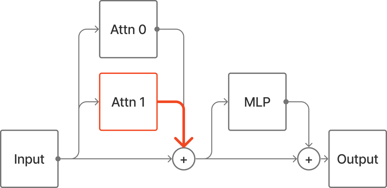
Node Patching (aka. “normal” activation patching) is when some activation in a neural network is altered from the value computed by the network to some other value. For example we could run two different prompts through a language model and replace the output of Attn 1 when the model is given some input 1 with the output of the head when the model is given some other input 2.

We will use the running example of a tiny, 1-layer transformer, but this approach generalizes to any transformer and any residual network.

All the nodes downstream of Attn 1 will be affected by the patch.

Edge Patching

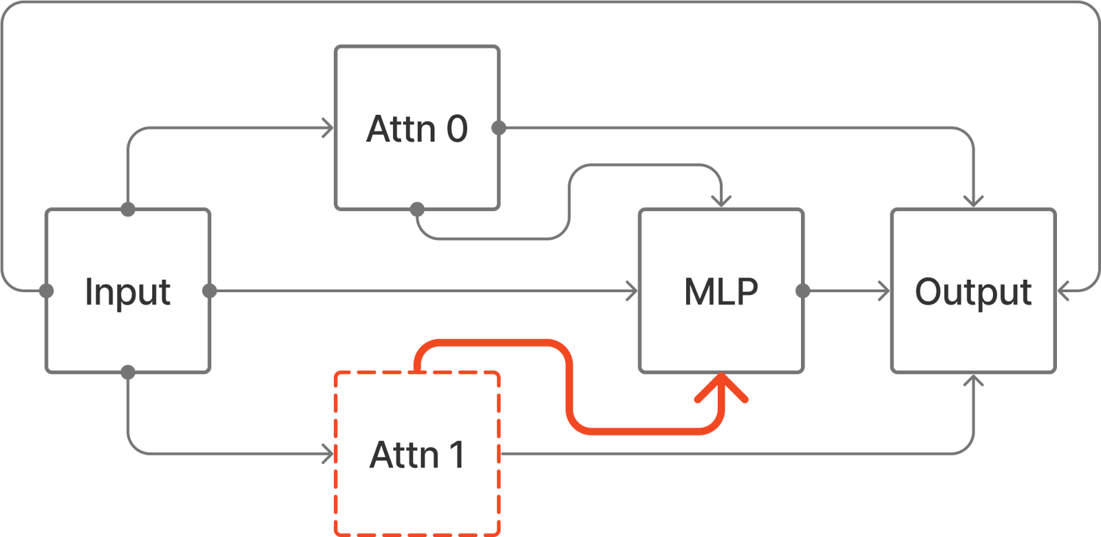
If we want to make a more precise intervention, we can think about the transformer differently, to isolate the interactions between components.

Now we can patch the edge Attn 1 -> MLP and only nodes downstream of MLP will be affected (eg. Attn 1->Output is unchanged). Edge Patching has not been explicitly named in any prior work.

Path Patching

Path Patching refers to the intervention where an input to a path is replaced in the ‘treeified’ view of the model. The treeified view is a third way of thinking about the model where we separate each path from input to output. We can implement an equivalent intervention to the previous diagram as follows:

In the IOI paper, ‘Path Patching’ the edge Component 1 -> Component 2 means Path Patching all paths of the form

Input -> ... -> Component 1 -> ... -> Component 2 -> ... -> Output

where all components between Component 1 and Component 2 are MLPs^[1]. However, it can be easy to confuse Edge Patching and Path Patching because if we instead patch all paths of the form

Input -> ... -> Component 1 -> Component 2 -> ... -> Output

this is equivalent to Edge Patching the edge Component 1->Component 2.

Edge Patching all of the edges which have some node as source is equivalent to Node Patching that node. AutoCircuit does not implement Path Patching, which is much more expensive in general. However, as explained in the appendix, Path Patching is sometimes equivalent to Edge Patching.

Fast Edge Patching

We perform two steps.

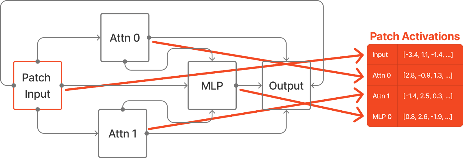
• First we gather the activations that we want to patch into the model. There’s many ways to do this, depending on what type of patching you want to do. If we just want to do zero ablation, then we don’t need to even run the model. But let’s assume we want to patch in activations from a different, corrupt input. We create a tensor, Patch Activations, to store the outputs of the source of each edge and we write to the tensor during the forward pass. Each source component has a row in the tensor, so the shape is [n_sources, batch, seq, d_model].^[2]

• Now we run the forward pass in which we actually do the patching. We write the outputs of each edge source to a different tensor, Current Activations, of the same shape as Patch Activations. When we get to the input of the destination component of the edge we want to patch, we add the difference between the rows of Patch Activations and Current Activations corresponding to the edge’s source component output.

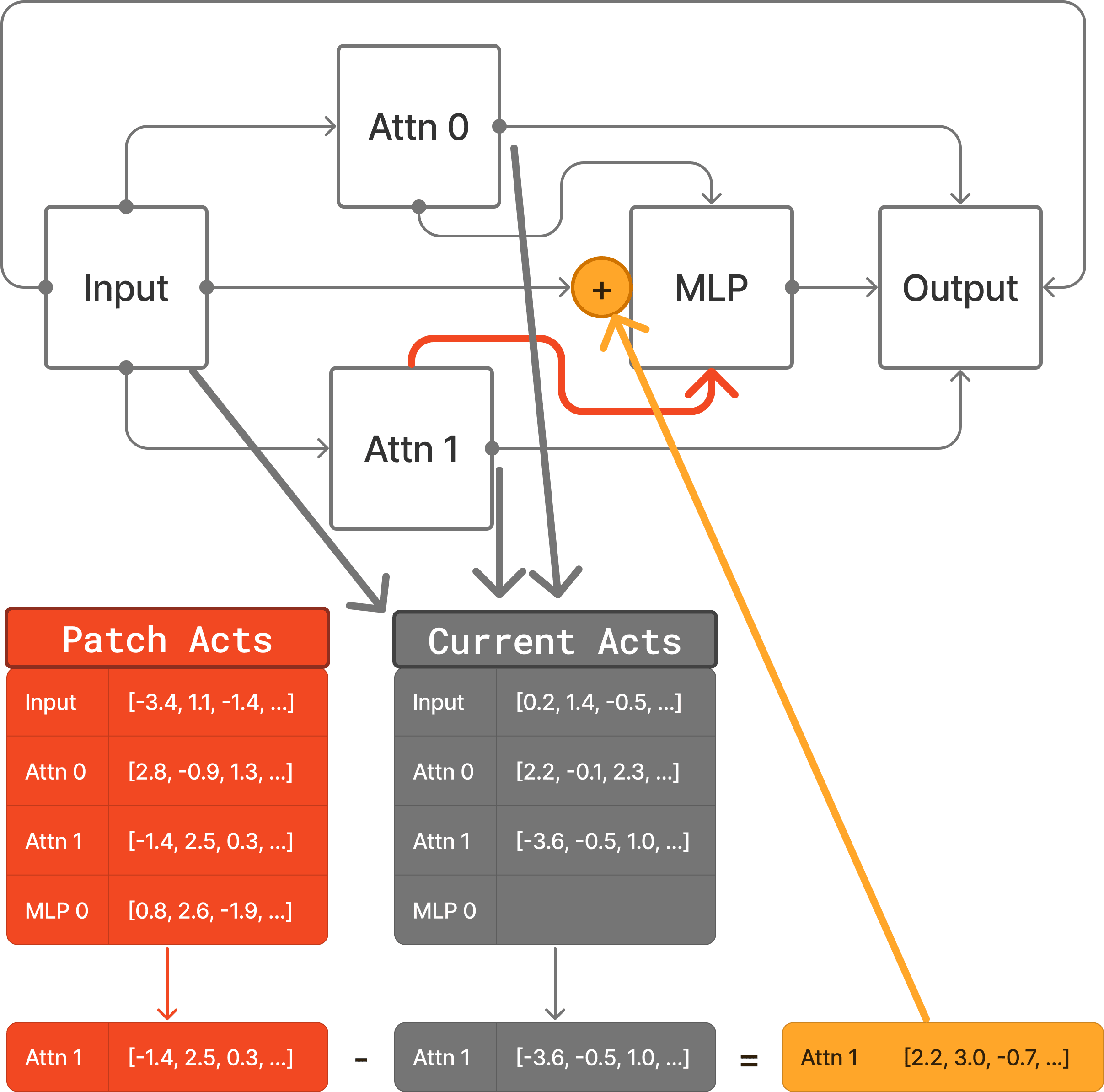
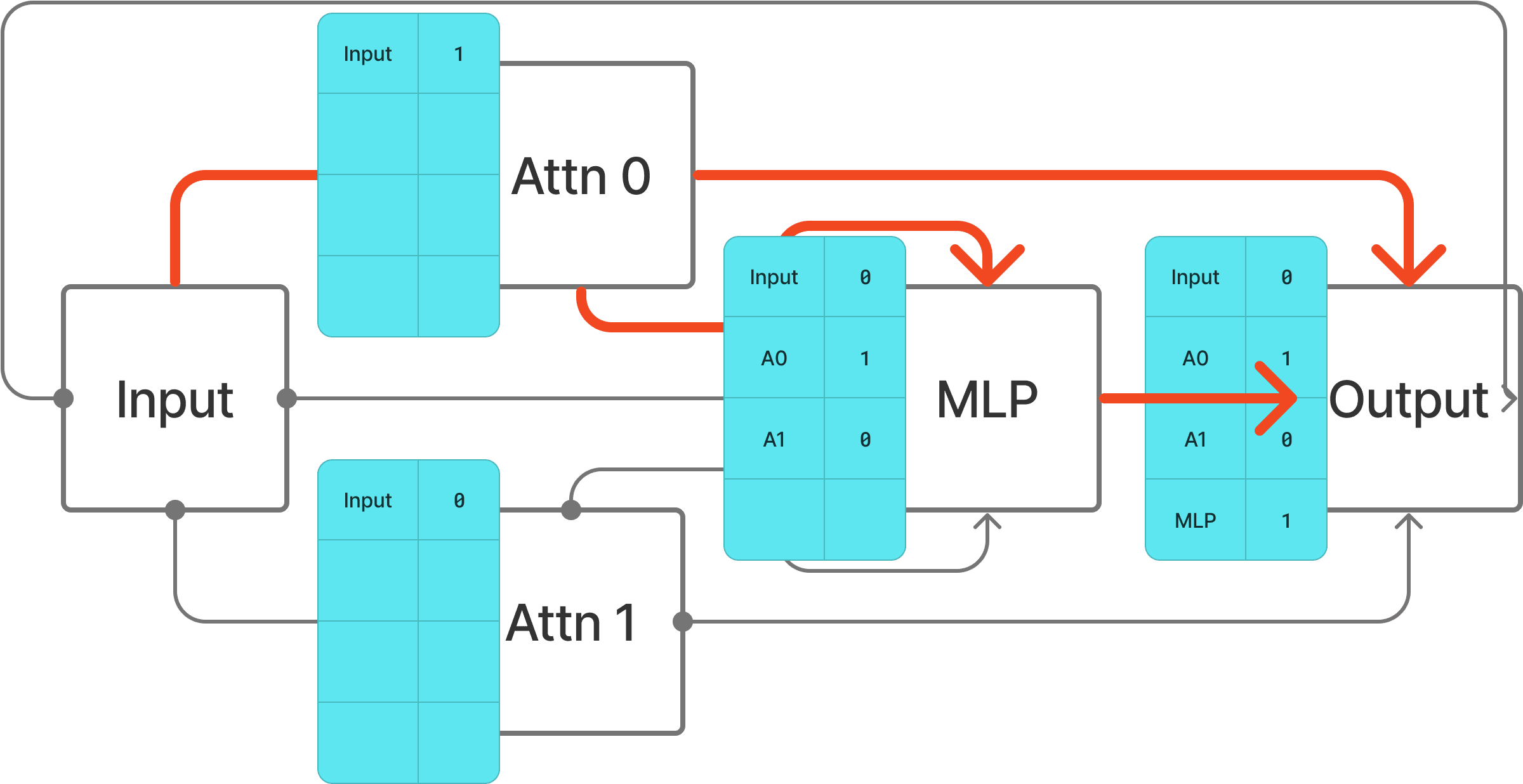
This works because the difference in input to the edge destination is equal to the difference in output of the source component.^[3] Now it’s straightforward to extend this to patching multiple edges at once by subtracting the entire Current Activations tensor from the entire Patch Activations tensor and multiplying by a Mask tensor of shape [n_sources] that has a single value for each input edge.

By creating a Mask tensor for each destination node we can patch any set of edges in the model. Crucially, the entire process is vectorized so it’s executed very efficiently on the GPU.

Performance Comparison

We test the performance using the ACDC circuit discovery algorithm, which iteratively patches every edge in the model. We compare the performance of AutoCircuit's implementation to the official ACDC hook-based implementation. We run ACDC using both libraries at a range of thresholds for a tiny 2-layer model with only 0.5 million parameters^[4] and measure the time taken to execute.^[5]

Different numbers of edges are included at different thresholds in the ACDC algorithm.^[6] While this greatly affects the performance of the hook-based implementation, it doesn't change the fast implementation because mask parameters for all edges are always included.

Mask Gradients

In AutoCircuit, masks are implemented not using hooks, but by injecting new PyTorch Modules that wrap the existing node modules and perform the Edge Patching. The Mask tensors are Parameters of the wrapper Modules. This means that we can compute the gradients of the model output with respect to the Mask values using the normal AutoGrad system.

So we can ‘train’ a circuit by optimizing the Mask parameters using gradient descent^[7]. We can also compute the attribution of each edge very easily. If we set all Masks to 0, the attribution is simply the gradient of output with respect to the mask.

Proof:

Let $\alpha \in [0,1]$ interpolate between the clean and corrupt edge activation $e_{\text{clean}}$ and $e_{\text{corr}}$:

$e_{\alpha }=e_{\text{clean}}+\alpha \times (e_{\text{corr}}-e_{\text{clean}})$

Then

$\frac{\partial F\left(e_{\alpha }\right)}{\partial \alpha }=\frac{\partial F\left(e_{\alpha }\right)}{\partial e_{\alpha }}\frac{\partial e_{\alpha }}{\partial \alpha }$

$=\frac{\partial F\left(e_{\alpha }\right)}{\partial e_{\alpha }}\frac{\partial [e_{\text{clean}}+\alpha \times (e_{\text{corr}}-e_{\text{clean}}\left)\right]}{\partial \alpha }$

$=\frac{\partial F\left(e_{\alpha }\right)}{\partial e_{\alpha }}{e}_{\text{corr}}-e_{\text{clean}}$

Set $\alpha =0$, ie. $e_{\alpha }=e_{clean}$

$=e_{\text{corr}}-e_{\text{clean}}\frac{\partial F\left(e_{\text{clean}}\right)}{\partial e_{\text{clean}}}$

Which is the definition of (edge) attribution patching.

Intuition:

The gradient of the output with respect to the activation is the amount that the output would change if you add $\delta x$ to the activation, divided by $\delta x$. So we need to multiply by $e_{\text{corr}}-e_{\text{clean}}$ to estimate the effect of patching.

The gradient of the output with respect to the mask is the amount that the output would change if you add $\delta x\times (e_{\text{corr}}-e_{\text{clean}})$ to the activation, divided by $\delta x$. So the full effect of patching is already accounted for.

Appendix: Path Patching vs. Edge Patching

In general 'treeified' interventions have time complexity exponential in the number of layers of the model, because each node sees a different “copy” than its siblings of the subtree upstream of itself, and each copy can have different inputs. However, there is a special class of treeified interventions which can be implemented using Edge Patching.

Starting with a simple example, we have already seen that the path

Input -> Attn 1 -> MLP -> Output

can be patched by Edge Patching the edge Attn 1 -> MLP.

Now consider a transformer with an extra attention layer.

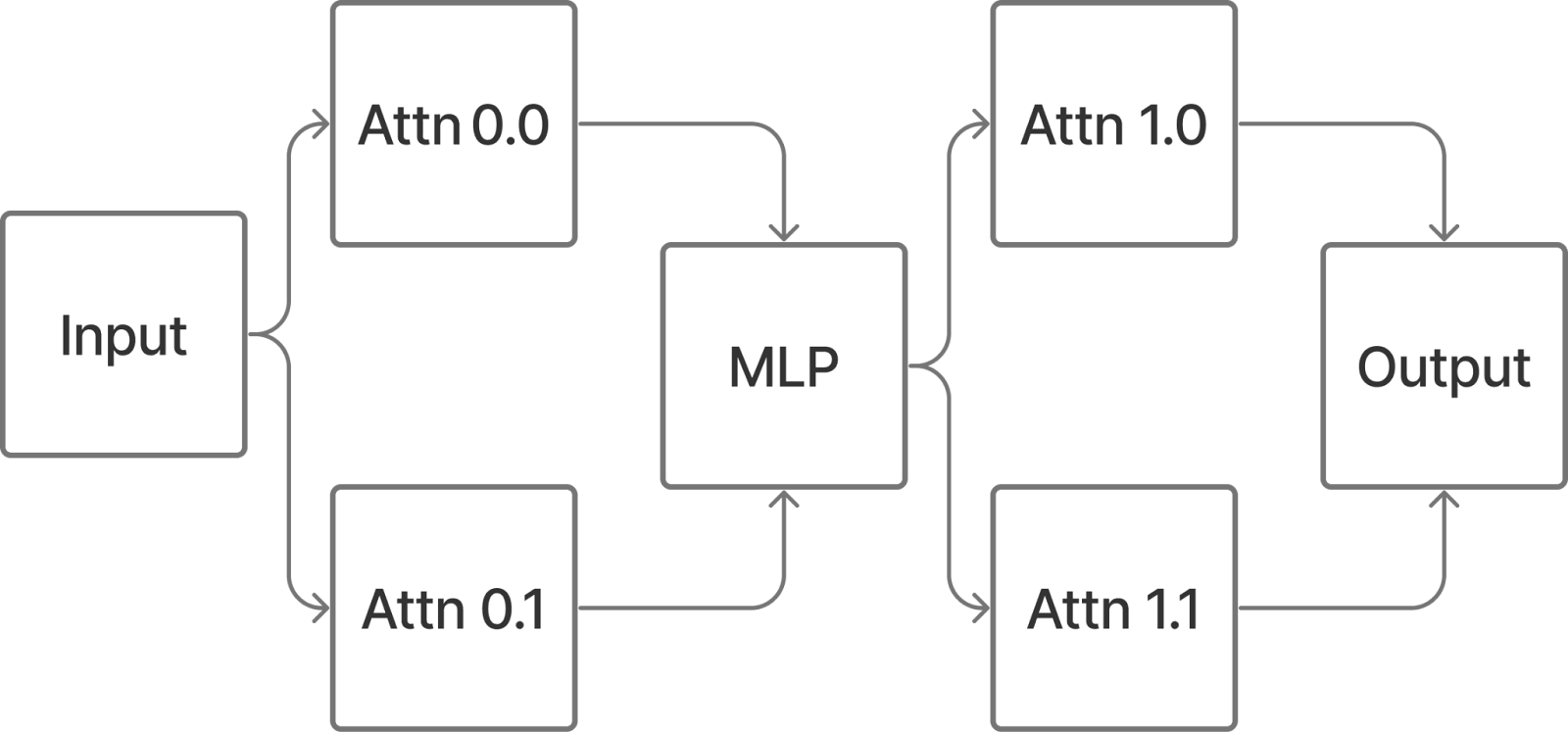
Say we want to patch the path

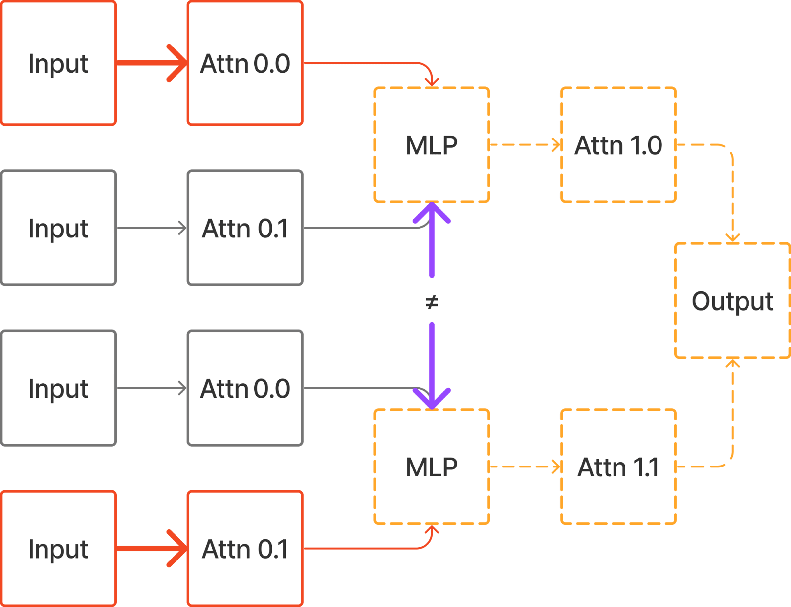
Input -> Attn 0.0 -> MLP -> Attn 1.0 -> Output

This can be implemented in the treefied view with Path Patching as follows:

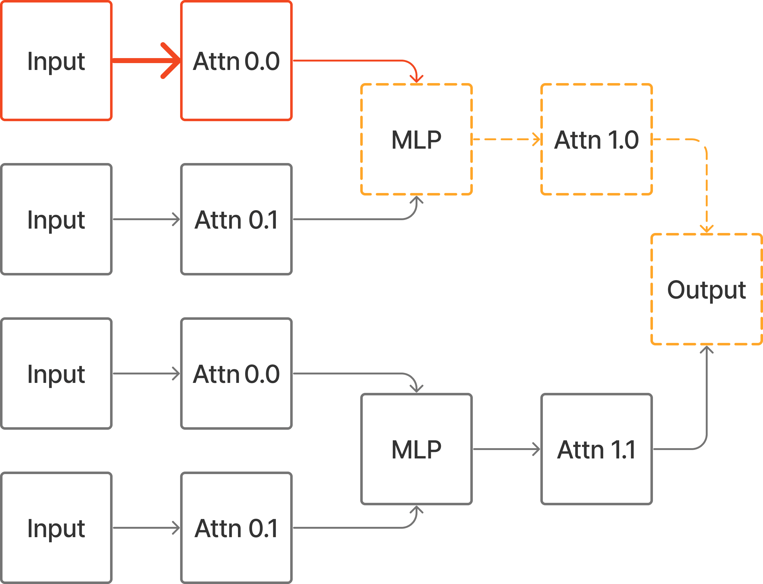
However, if we just Edge Patch Attn 0.0 -> MLP (or Input -> Attn 0.0), we will get a different output because there is a downstream effect on Attn 1.1.

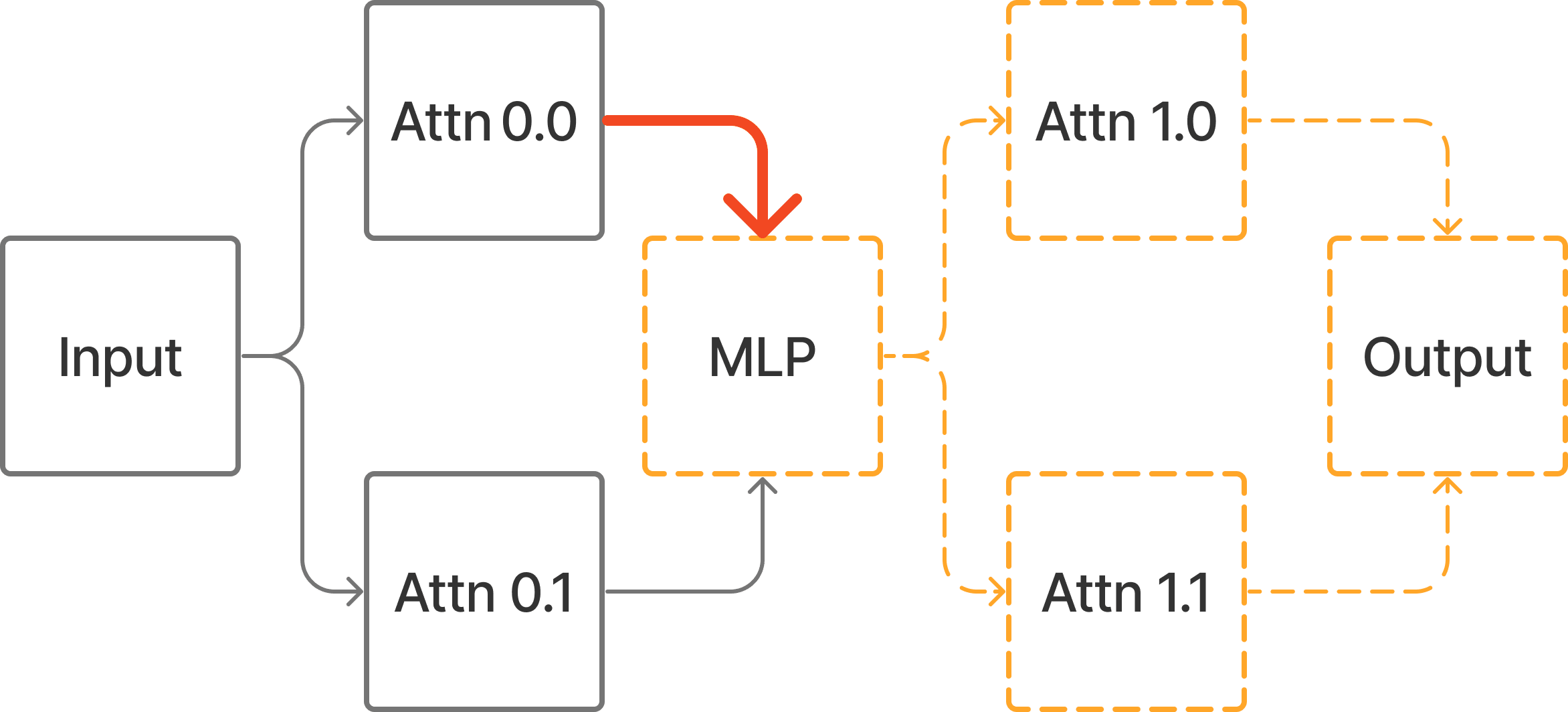
If we instead change the input to the corrupt prompt and patch in clean activations to the complement of the circuit, then we can achieve the desired intervention.

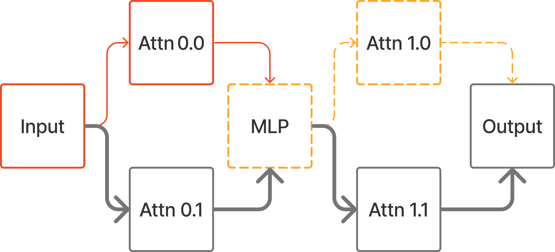
In general, Edge Patching can be used to implement any treeified hypothesis in which all instances of a node have the same input. This means that any Causal Scrubbing [AF · GW] hypothesis which just specifies a set of important and unimportant edges (and a single clean and corrupt prompt pair) can be implemented with fast Edge Patching.

But a circuit hypothesis which specifies a set of important and unimportant paths cannot always be implemented with Edge Patching. 

For example, if we want to patch the paths

Input -> Attn 0.0 -> MLP -> Attn 1.0 -> Output
Input -> Attn 0.1 -> MLP -> Attn 1.1 -> Output

this can only be expressed in the treeified model, because it requires the output of the MLP to be computed on two different inputs, and for both outputs of the MLP to be propagated to the output.

Thanks to Bilal Chughtai for his extensive feedback. Thanks to Nix Goldowsky-Dill and Arthur Conmy for their comments. Thanks to Sam Marks for the example of a treeified intervention that cannot be implemented by Edge Patching.

1. ^{^}

   They hypothesize that the task is mostly performed by attention heads, at it only requires moving information around.

2. ^{^}

   n_sources is the number of source nodes in the model. batch is the number of elements in the current input batch. seq is the length of the prompts in the batch. d_model is the size of the model activations.

3. ^{^}

   This will always be the case for the edges in this diagram, but it won’t work if you consider MLPs to be included in the direct edges between attention heads, as they do in the IOI paper (which is why that is Path Patching, not Edge Patching).

4. ^{^}

   For larger models, both implementations will take longer to execute. The ratio of execution time between the two probably remains similar. But ACDC becomes sufficiently slow that this is annoying to test for eg. >50% of edges included in GPT-2, so we're not certain what the curve looks like.

5. ^{^}

   Note that the AutoCircuit library contains other optimizations besides the fasting patching method. In particular, in the ACDC algorithm we cache layers during forward passes that patch edges to nodes in later layers.

   So this is not a fair comparison for measuring the speedup from the fast patching method alone. However, the ACDC repo is the most popular library for patching and the ACDC algorithm is one of the most common use-cases where you would want to patch most of the edges in a model so it seems like a useful metric anyway.

6. ^{^}

   Note that ACDC and AutoCircuit count the number of edges differently (AutoCircuit doesn't include 'Direct Computation' or 'Placeholder' edges) so we compare the proportion of edges included. The underlying computation graphs are equivalent.

7. ^{^}

   Also done by Li et al. (2023).

8. ^{^}

   Note that the AutoCircuit library contains other optimizations besides the fasting patching method. In particular, we cache layers during forward passes that patch edges to nodes in later layers.

   So this is not a fair comparison for measuring the speedup from the fast patching method alone. However, the ACDC repo is the most popular library for patching and the ACDC algorithm is one of the few use-cases where you would want to patch most of the edges in a model so it seems like a useful metric anyway.

6 comments

Comments sorted by top scores.