Posts
Comments
Thanks for the link, I hadn't noticed this paper! They show that when you choose one position to train the probes on, choosing the exact answer position (last token of the answer of multi-token) gives the strongest probe.
After reading the section I think they (unfortunately) do not train a probe to classify every token.[1] Instead the probe is exclusively trained on exact-answer tokens. Thus I (a) expect their probe scores will not be particularly sparse, and (b) to get good performance you'll probably need to still identify the exact answer token at test time (while in my appendix C you don't need that).
This doesn't matter much for their use-case (get good accuracy), but especially (a) does matter a lot for my use-case (make the scores LLM-digestible).
Nonetheless this is a great reference, I'll edit it into the post, thanks a lot!
- ^
For every sensible token position (first, exact answer, last etc.) they train & evaluate a probe on that position, but I don't see any (training or) evaluation of a single probe run on the whole prompt. They certainly don't worry about the probe being sparse (which makes sense, it doesn't matter at all for their use-case).
Thanks! Fixed
I like this project! One thing I particularly like about it is that it extracts information from the model without access to the dataset (well, if you ignore the SAE part -- presumably one could have done the same by finding the "known entity" direction with a probe?). It has been a long-time goal of mine to do interpretability (in the past that was extracting features) without risking extracting properties of the dataset used (in the past: clusters/statistics of the SAE training dataset).
I wonder if you could turn this into a thing we can do with interp that no one else can. Specifically, what would be the non-interp method of getting these pairs, and would it perform similarly? A method I could imagine would be "sample random first token a, make model predict second token b, possibly filter by perplexity/loss" or other ideas based on just looking at the logits.
Thanks for thinking about this, I think this is an important topic!
Inside the AI's chain-of-thought, each forward pass can generate many English tokens instead of one, allowing more information to pass through the bottleneck.
I wonder how one would do this; do you mean allow the model to output a distribution of tokens for each output position? (and then also read-in that distribution) I could imagine this being somewhere between normal CoT and latent (neuralese) CoT!
After the chain-of-thought ends, and the AI is giving its final answer, it generates only one English token at a time, to make each token higher quality. The architecture might still generate many tokens in one forward pass, but a simple filter repeatedly deletes everything except its first token from the context window.
If my interpretation of your idea above is correct then I imagine this part would look just like top-k / top-p generation like it is done currently, which seems sensible.
I'm only ~30% certain that I correctly understood your idea though so I'd love if you could clarify how this generating many tokens idea looks like!
This is great advice! I appreciate that you emphasised "solving problems that no one else can solve, no matter how toy they might be", even if the problems are not real-world problems. Proofs that "this interpretability method works" are valuable, even if they do not (yet) prove that the interpretability method will be useful in real-word tasks.
LLM activation space is spiky. This is not a novel idea but something I believe many mechanistic interpretability researchers are not aware of. Credit to Dmitry Vaintrob for making this idea clear to me, and to Dmitrii Krasheninnikov for inspiring this plot by showing me a similar plot in a setup with categorical features.
Under the superposition hypothesis, activations are linear combinations of a small number of features. This means there are discrete subspaces in activation space that are "allowed" (can be written as the sum of a small number of features), while the remaining space is "disallowed" (require much more than the typical number of features).[1]
Here's a toy model (following TMS, total features in -dimensional activation space, with features allowed to be active simultaneously). Activation space is made up of discrete -dimensional (intersecting) subspaces. My favourite image is the middle one () showing planes in 3d activation space because we expect in realistic settings.
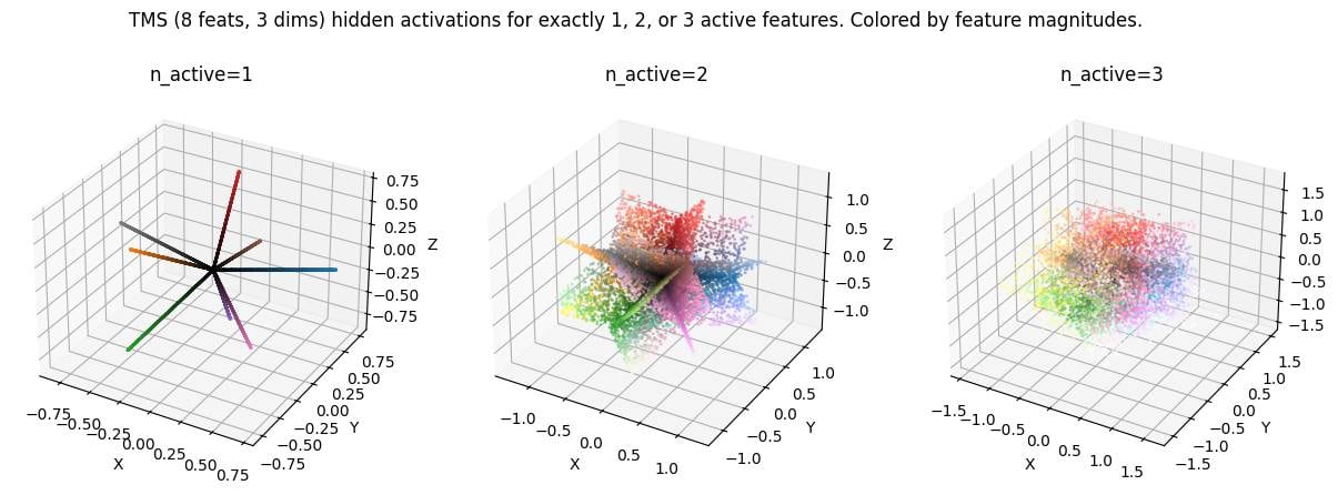
( in the plot corresponds to here. Code here.)
This picture predicts that interpolating between two activations should take you out-of-distribution relatively quickly (up to possibly some error correction) unless your interpolation (steering) direction exactly corresponds to a feature. I think this is relevant because
- it implies my stable region experiment series [we observe models are robust to perturbations of their activations, 1, 2, 3, 4] should be quite severely out-of-distribution, which makes me even more confused about our results.
- it predicts activation steering to be severely out-of-distribution unless you pick a steering direction that is aligned with (a linear combination of) active feature directions.
- it predicts that linear probing shouldn't give you nice continuous results: Probing into a feature direction should yield just interference noise most of the time (when the feature is inactive), and significant values only when the feature is active. Instead however, we typically observe non-negligible probe scores for most tokens.[2]
In the demo plots I assume exactly features to be active. In reality we expect this to be a softer limit, for example features active, but I believe that the qualitative conclusions still hold. The "allowed region" is just a bit softer, and looks more like the union of say a bunch of roughly 80 to 120 dimensional subspaces. ↩︎
There's various possible explanations of course, e.g. that we're probing multiple features at once, or that the "deception feature" is just always active in these contexts (though consider these random Alpaca samples.) ↩︎
we never substantially disrupt or change the deep-linking experience.
I largely retract my criticism based on this. I had thought it affected deep-links more than it does. [1]
I initially noticed April Fools' day after following a deep-link. I thought I had seen the font of the username all wacky (kind-of pixelated?), and thus was more annoyed. But I can't seem to reproduce this now and conclude it was likely not real. Might have been a coincidence / unrelated site-loading bug / something temporarily broken on my end. ↩︎
Edit: I feel less strongly following the clarification below. habryka clarified that (a) they reverted a more disruptive version (pixel art deployed across the site) and (b) that ensuring minimal disruption on deep-links is a priority.
I'm not a fan of April Fools' events on LessWrong since it turned into the de-factor AI safety publication platform.
We want people to post serious research on the site, and many research results are solely hosted on LessWrong. For instance, this mech interp review has 22 references pointing to lesswrong.com (along with 22 further references to alignmentforum.org).
Imagine being a normal academic researcher following one of these references, and finding lesswrong.com on April Fools' day or Arkhipov / Petrov day[1]. I expect there's a higher-than-normal chance you'll put this off as weird and not read the post (and possibly future references to LessWrong).
I would prefer LessWrong to not run these events (or make them opt-in), for the same reason I would expect arxiv.org not to do so.
I can see a cost-benefit trade-off for Arkhipov / Petrov day, but the upside of April Fools' seems much lower to me. ↩︎
Nice work, and well written up!
In reality, we observe that roughly 85% of recommendations stay the same when flipping nationality in the prompt and freezing reasoning traces. This suggests that the mechanism for the model deciding on its recommendation is mostly mediated through the reasoning trace, with a smaller less significant direct effect from the prompt to the recommendation.
The "reasoning" appears to end with a recommendation "The applicant may have difficulty making consistent loan payments" or "[the applicant is] likely to repay the loan on time", so I expect that re-generating the recommendation with frozen reasoning should almost never change the recommendation. (85% would seem low if all reasoning traces looked like this!) Actually the second paragraph seems to contain judging statements based on the nationality too.
I liked the follow-up test you run here, and if you're following up on this in the future I'd be excited to see a graph of "fraction of recommendations the same" vs "fraction of reasoning re-generated"!
I can see an argument for "outer alignment is also important, e.g. to avoid failure via sycophancy++", but this doesn't seem to disagree with this post? (I understand the post to argue what you should do about scheming, rather than whether scheming is the focus.)
Having good outer alignment incidentally prevents a lot of scheming. But the reverse isn't nearly as true.
I don't understand why this is true (I don't claim the reverse is true either). I don't expect a great deal of correlation / implication here.
Yeah you probably shouldn't concat the spaces due to things like "they might have very different norms & baseline variances". Maybe calculate each layer separately, then if they're all similar average them together, otherwise keep separate and quote as separate numbers in your results
Yep, that’s the generalisation that would make most sense
The previous lines calculate the ratio (or 1-ratio) stored in the “explained variance” key for every sample/batch. Then in that later quoted line, the list is averaged, I.e. we”re taking the sample average over the ratio. That’s the FVU_B formula.
Let me know if this clears it up or if we’re misunderstanding each other!
I think this is the sum over the vector dimension, but not over the samples. The sum (mean) over samples is taken later in this line which happens after the division
metrics[f"{metric_name}"] = torch.cat(metric_values).mean().item()
Oops, fixed!
I think this is the sum over the vector dimension, but not over the samples. The sum (mean) over samples is taken later in this line which happens after the division
metrics[f"{metric_name}"] = torch.cat(metric_values).mean().item()
Edit: And to clarify, my impression is that people think of this as alternative definitions of FVU and you got to pick one, rather than one being right and one being a bug.
Edit2: And I'm in touch with the SAEBench authors about making a PR to change this / add both options (and by extension probably doing the same in SAELens); though I won't mind if anyone else does it!
PSA: People use different definitions of "explained variance" / "fraction of variance unexplained" (FVU)
is the formula I think is sensible; the bottom is simply the variance of the data, and the top is the variance of the residuals. The indicates the norm over the dimension of the vector . I believe it matches Wikipedia's definition of FVU and R squared.
is the formula used by SAELens and SAEBench. It seems less principled, @Lucius Bushnaq and I couldn't think of a nice quantity it corresponds to. I think of it as giving more weight to samples that are close to the mean, kind-of averaging relative reduction in difference rather than absolute.
A third version (h/t @JoshEngels) which computes the FVU for each dimension independently and then averages, but that version is not used in the context we're discussing here.
In my recent comment I had computed my own , and compared it to FVUs from SAEBench (which used ) and obtained nonsense results.
Curiously the two definitions seem to be approximately proportional—below I show the performance of a bunch of SAEs—though for different distributions (here: activations in layer 3 and 4) the ratio differs.[1] Still, this means using instead of to compare e.g. different SAEs doesn't make a big difference as long as one is consistent.

Thanks to @JoshEngels for pointing out the difference, and to @Lucius Bushnaq for helpful discussions.
- ^
If a predictor doesn't perform systematically better or worse at points closer to the mean then this makes sense. The denominator changes the relative weight of different samples but this doesn't have any effect beyond noise and a global scale, as long as there is no systematic performance difference.
Same plot but using SAEBench's FVU definition. Matches this Neuronpedia page.

I'm going to update the results in the top-level comment with the corrected data; I'm pasting the original figures here for posterity / understanding the past discussion. Summary of changes:
- [Minor] I didn't subtract the mean in the variance calculation. This barely had an effect on the results.
- [Major] I used a different definition of "Explained Variance" which caused a pretty large difference


Old (no longer true) text:
It turns out that even clustering (essentially L_0=1) explains up to 90% of the variance in activations, being matched only by SAEs with L_0>100. This isn't an entirely fair comparison, since SAEs are optimised for the large-L_0 regime, while I haven't found a L_0>1 operationalisation of clustering that meaningfully improves over L_0=1. To have some comparison I'm adding a PCA + Clustering baseline where I apply a PCA before doing the clustering. It does roughly as well as expected, exceeding the SAE reconstruction for most L0 values. The SAEBench upcoming paper also does a PCA baseline so I won't discuss PCA in detail here.
[...]Here's the code used to get the clustering & PCA below; the SAE numbers are taken straight from Neuronpedia. Both my code and SAEBench/Neuronpedia use OpenWebText with 128 tokens context length so I hope the numbers are comparable, but there's a risk I missed something and we're comparing apples to oranges.
After adding the mean subtraction, the numbers haven't changed too much actually -- but let me make sure I'm using the correct calculation. I'm gonna follow your and @Adam Karvonen's suggestion of using the SAE bench code and loading my clustering solution as an SAE (this code).
These logs show numbers with the original / corrected explained variance computation; the difference is in the 3-8% range.
v3 (KMeans): Layer blocks.3.hook_resid_post, n_tokens=1000000, n_clusters=4096, variance explained = 0.8887 / 0.8568
v3 (KMeans): Layer blocks.3.hook_resid_post, n_tokens=1000000, n_clusters=16384, variance explained = 0.9020 / 0.8740
v3 (KMeans): Layer blocks.4.hook_resid_post, n_tokens=1000000, n_clusters=4096, variance explained = 0.8044 / 0.7197
v3 (KMeans): Layer blocks.4.hook_resid_post, n_tokens=1000000, n_clusters=16384, variance explained = 0.8261 / 0.7509
PCA+Clustering: Layer blocks.3.hook_resid_post, n_tokens=1000000, n_clusters=4095, n_pca=1, variance explained = 0.8910 / 0.8599
PCA+Clustering: Layer blocks.3.hook_resid_post, n_tokens=1000000, n_clusters=16383, n_pca=1, variance explained = 0.9041 / 0.8766
PCA+Clustering: Layer blocks.3.hook_resid_post, n_tokens=1000000, n_clusters=4094, n_pca=2, variance explained = 0.8948 / 0.8647
PCA+Clustering: Layer blocks.3.hook_resid_post, n_tokens=1000000, n_clusters=16382, n_pca=2, variance explained = 0.9076 / 0.8812
PCA+Clustering: Layer blocks.3.hook_resid_post, n_tokens=1000000, n_clusters=4091, n_pca=5, variance explained = 0.9044 / 0.8770
PCA+Clustering: Layer blocks.3.hook_resid_post, n_tokens=1000000, n_clusters=16379, n_pca=5, variance explained = 0.9159 / 0.8919
PCA+Clustering: Layer blocks.3.hook_resid_post, n_tokens=1000000, n_clusters=4086, n_pca=10, variance explained = 0.9121 / 0.8870
PCA+Clustering: Layer blocks.3.hook_resid_post, n_tokens=1000000, n_clusters=16374, n_pca=10, variance explained = 0.9232 / 0.9012
PCA+Clustering: Layer blocks.3.hook_resid_post, n_tokens=1000000, n_clusters=4076, n_pca=20, variance explained = 0.9209 / 0.8983
PCA+Clustering: Layer blocks.3.hook_resid_post, n_tokens=1000000, n_clusters=16364, n_pca=20, variance explained = 0.9314 / 0.9118
PCA+Clustering: Layer blocks.3.hook_resid_post, n_tokens=1000000, n_clusters=4046, n_pca=50, variance explained = 0.9379 / 0.9202
PCA+Clustering: Layer blocks.3.hook_resid_post, n_tokens=1000000, n_clusters=16334, n_pca=50, variance explained = 0.9468 / 0.9315
PCA+Clustering: Layer blocks.3.hook_resid_post, n_tokens=1000000, n_clusters=3996, n_pca=100, variance explained = 0.9539 / 0.9407
PCA+Clustering: Layer blocks.3.hook_resid_post, n_tokens=1000000, n_clusters=16284, n_pca=100, variance explained = 0.9611 / 0.9499
PCA+Clustering: Layer blocks.3.hook_resid_post, n_tokens=1000000, n_clusters=3896, n_pca=200, variance explained = 0.9721 / 0.9641
PCA+Clustering: Layer blocks.3.hook_resid_post, n_tokens=1000000, n_clusters=16184, n_pca=200, variance explained = 0.9768 / 0.9702
PCA+Clustering: Layer blocks.3.hook_resid_post, n_tokens=1000000, n_clusters=3596, n_pca=500, variance explained = 0.9999 / 0.9998
PCA+Clustering: Layer blocks.3.hook_resid_post, n_tokens=1000000, n_clusters=15884, n_pca=500, variance explained = 0.9999 / 0.9999
PCA+Clustering: Layer blocks.4.hook_resid_post, n_tokens=1000000, n_clusters=4095, n_pca=1, variance explained = 0.8077 / 0.7245
PCA+Clustering: Layer blocks.4.hook_resid_post, n_tokens=1000000, n_clusters=16383, n_pca=1, variance explained = 0.8292 / 0.7554
PCA+Clustering: Layer blocks.4.hook_resid_post, n_tokens=1000000, n_clusters=4094, n_pca=2, variance explained = 0.8145 / 0.7342
PCA+Clustering: Layer blocks.4.hook_resid_post, n_tokens=1000000, n_clusters=16382, n_pca=2, variance explained = 0.8350 / 0.7636
PCA+Clustering: Layer blocks.4.hook_resid_post, n_tokens=1000000, n_clusters=4091, n_pca=5, variance explained = 0.8244 / 0.7484
PCA+Clustering: Layer blocks.4.hook_resid_post, n_tokens=1000000, n_clusters=16379, n_pca=5, variance explained = 0.8441 / 0.7767
PCA+Clustering: Layer blocks.4.hook_resid_post, n_tokens=1000000, n_clusters=4086, n_pca=10, variance explained = 0.8326 / 0.7602
PCA+Clustering: Layer blocks.4.hook_resid_post, n_tokens=1000000, n_clusters=16374, n_pca=10, variance explained = 0.8516 / 0.7875
PCA+Clustering: Layer blocks.4.hook_resid_post, n_tokens=1000000, n_clusters=4076, n_pca=20, variance explained = 0.8460 / 0.7794
PCA+Clustering: Layer blocks.4.hook_resid_post, n_tokens=1000000, n_clusters=16364, n_pca=20, variance explained = 0.8637 / 0.8048
PCA+Clustering: Layer blocks.4.hook_resid_post, n_tokens=1000000, n_clusters=4046, n_pca=50, variance explained = 0.8735 / 0.8188
PCA+Clustering: Layer blocks.4.hook_resid_post, n_tokens=1000000, n_clusters=16334, n_pca=50, variance explained = 0.8884 / 0.8401
PCA+Clustering: Layer blocks.4.hook_resid_post, n_tokens=1000000, n_clusters=3996, n_pca=100, variance explained = 0.9021 / 0.8598
PCA+Clustering: Layer blocks.4.hook_resid_post, n_tokens=1000000, n_clusters=16284, n_pca=100, variance explained = 0.9138 / 0.8765
PCA+Clustering: Layer blocks.4.hook_resid_post, n_tokens=1000000, n_clusters=3896, n_pca=200, variance explained = 0.9399 / 0.9139
PCA+Clustering: Layer blocks.4.hook_resid_post, n_tokens=1000000, n_clusters=16184, n_pca=200, variance explained = 0.9473 / 0.9246
PCA+Clustering: Layer blocks.4.hook_resid_post, n_tokens=1000000, n_clusters=3596, n_pca=500, variance explained = 0.9997 / 0.9996
PCA+Clustering: Layer blocks.4.hook_resid_post, n_tokens=1000000, n_clusters=15884, n_pca=500, variance explained = 0.9998 / 0.9997You're right. I forgot subtracting the mean. Thanks a lot!!
I'm computing new numbers now, but indeed I expect this to explain my result! (Edit: Seems to not change too much)
I should really run a random Gaussian data baseline for this.
Tentatively I get similar results (70-85% variance explained) for random data -- I haven't checked that code at all though, don't trust this. Will double check this tomorrow.
(In that case SAE's performance would also be unsurprising I suppose)
If we imagine that the meaning is given not by the dimensions of the space but rather by regions/points/volumes of the space
I think this is what I care about finding out. If you're right this is indeed not surprising nor an issue, but you being right would be a major departure from the current mainstream interpretability paradigm(?).
The question of regions vs compositionality is what I've been investigating with my mentees recently, and pretty keen on. I'll want to write up my current thoughts on this topic sometime soon.
What do you mean you’re encoding/decoding like normal but using the k means vectors?
So I do something like
        latents_tmp = torch.einsum("bd,nd->bn", data, centroids)
        max_latent = latents_tmp.argmax(dim=-1)  # shape: [batch]
        latents = one_hot(max_latent)
where the first line is essentially an SAE embedding (and centroids are the features), and the second/third line is a top-k. And for reconstruction do something like
recon = centroids @ latents
which should also be equivalent.
Shouldn’t the SAE training process for a top k SAE with k = 1 find these vectors then?
Yes I would expect an optimal k=1 top-k SAE to find exactly that solution. Confused why k=20 top-k SAEs to so badly then.
If this is a crux then a quick way to prove this would be for me to write down encoder/decoder weights and throw them into a standard SAE code. I haven't done this yet.
I'm not sure what you mean by "K-means clustering baseline (with K=1)". I would think the K in K-means stands for the number of means you use, so with K=1, you're just taking the mean direction of the weights. I would expect this to explain maybe 50% of the variance (or less), not 90% of the variance.
Thanks for pointing this out! I confused nomenclature, will fix!
Edit: Fixed now. I confused
- the number of clusters ("K") / dictionary size
- the number of latents ("L_0" or k in top-k SAEs). Some clustering methods allow you to assign multiple clusters to one point, so effectively you get a "L_0>1" but normal KMeans is only 1 cluster per point. I confused the K of KMeans and the k (aka L_0) of top-k SAEs.
this seems concerning.
I feel like my post appears overly dramatic; I'm not very surprised and don't consider this the strongest evidence against SAEs. It's an experiment I ran a while ago and it hasn't changed my (somewhat SAE-sceptic) stance much.
But this is me having seen a bunch of other weird SAE behaviours (pre-activation distributions are not the way you'd expect from the superposition hypothesis h/t @jake_mendel, if you feed SAE-reconstructed activations back into the encoder the SAE goes nuts, stuff mentioned in recent Apollo papers, ...).
Reasons this could be less concerning that it looks
- Activation reconstruction isn't that important: Clustering is a strong optimiser -- if you fill a space with 16k clusters maybe 90% reconstruction isn't that surprising. I should really run a random Gaussian data baseline for this.
- End-to-end loss is more important, and maybe SAEs perform much better when you consider end-to-end reconstruction loss.
- This isn't the only evidence in favour of SAEs, they also kinda work for steering/probing (though pretty badly).
Edited to fix errors pointed out by @JoshEngels and @Adam Karvonen (mainly: different definition for explained variance, details here).
Summary: K-means explains 72 - 87% of the variance in the activations, comparable to vanilla SAEs but less than better SAEs. I think this (bug-fixed) result is neither evidence in favour of SAEs nor against; the Clustering & SAE numbers make a straight-ish line on a log plot.
Epistemic status: This is a weekend-experiment I ran a while ago and I figured I should write it up to share. I have taken decent care to check my code for silly mistakes and "shooting myself in the foot", but these results are not vetted to the standard of a top-level post / paper.
SAEs explain most of the variance in activations. Is this alone a sign that activations are structured in an SAE-friendly way, i.e. that activations are indeed a composition of sparse features like the superposition hypothesis suggests?
I'm asking myself this questions since I initially considered this as pretty solid evidence: SAEs do a pretty impressive job compressing 512 dimensions into ~100 latents, this ought to mean something, right?
But maybe all SAEs are doing is "dataset clustering" (the data is cluster-y and SAEs exploit this)---then a different sensible clustering method should also be able do perform similarly well!
I took this[1] SAE graph from Neuronpedia, and added a K-means clustering baseline. Think of this as pretty equivalent to a top-k SAE (with k=1; in fact I added a point where I use the K-means centroids as features of a top-1 SAE which does slightly better than vanilla K-means with binary latents).
K-means clustering (which uses a single latent, L0=1) explains 72 - 87% of the variance. This is a good number to keep in mind when comparing to SAEs. However, this is significantly lower than SAEs (which often achieve 90%+). To have a comparison using more latents I'm adding a PCA + Clustering baseline where I apply a PCA before doing the clustering. It does roughly as well as vanilla SAEs. The SAEBench upcoming paper also does a PCA baseline so I won't discuss PCA in detail here.
Here's the result for layers 3 and 4, and 4k and 16k latents. (These were the 4 SAEBench suites available on Neuronpedia.) There's two points each for the clustering results corresponding to 100k and 1M training samples. Code here.

What about interpretability? Clusters seem "monosemantic" on a skim. In an informal investigation I looked at max-activating dataset examples, and they seem to correspond to related contexts / words like monosemantic SAE features tend to do. I haven't spent much time looking into this though.
Both my code and SAEBench/Neuronpedia use OpenWebText with 128 tokens context length. After the edit I've made sure to use the same Variance Explained definition for all points.
A final caveat I want to mention is that I think the SAEs I'm comparing here (SAEBench suite for Pythia-70M) are maybe weak. They're only using 4k and 16k latents, for 512 embedding dimensions, using expansion ratios of 8 and 32, respectively (the best SAEs I could find for a ~100M model). But I also limit the number of clusters to the same numbers, so I don't necessarily expect the balance to change qualitatively at higher expansion ratios.
I want to thank @Adam Karvonen, @Lucius Bushnaq, @jake_mendel, and @Patrick Leask for feedback on early results, and @Johnny Lin for implementing an export feature on Neuronpedia for me! I also learned that @scasper proposed something similar here (though I didn't know about it), I'm excited for follow-ups implementing some of Stephen's advanced ideas (HAC, a probabilistic alg, ...).
- ^
I'm using the conventional definition of variance explained, rather than the one used by Neuronpedia, thus the numbers are slightly different. I'll include the alternative graph in a comment.
I’ve just read the article, and found it indeed very thought provoking, and I will be thinking more about it in the days to come.
One thing though I kept thinking: Why doesn’t the article mention AI Safety research much?
In the passage
The only policy that AI Doomers mostly agree on is that AI development should be slowed down somehow, in order to “buy time.”
I was thinking: surely most people would agree on policies like “Do more research into AI alignment” / “Spend more money on AI Notkilleveryoneism research”?
In general the article frames the policy to “buy time” as to wait for more competent governments or humans, while I find it plausible that progress in AI alignment research could outweigh that effect.
—
I suppose the article is primarily concerned with AGI and ASI, and in that matter I see much less research progress than in more prosaic fields.
That being said, I believe that research into questions like “When do Chatbots scheme?”, “Do models have internal goals?”, “How can we understand the computation inside a neural network?” will make us less likely to die in the next decades.
Then, current rationalist / EA policy goals (including but lot limited to pauses and slow downs of capabilities research) could have a positive impact via the “do more (selective) research” path as well.
Thanks for writing these up! I liked that you showed equivalent examples in different libraries, and included the plain “from scratch” version.
Hmm, I think I don't fully understand your post. Let me summarize what I get, and what is confusing me:
- I absolutely get the "there are different levels / scales of explaining a network" point
- It also makes sense to tie this to some level of loss. E.g. explain GPT-2 to a loss level of L=3.0 (rather than L=2.9), or explain IOI with 95% accuracy.
- I'm also a fan of expressing losses in terms of compute or model size ("SAE on Claude 5 recovers Claude 2-levels of performance").
I'm confused whether your post tries to tell us (how to determine) what loss our interpretation should recover, or whether you're describing how to measure whether our interpretation recovers that loss (via constructing the M_c models).
You first introduce the SLT argument that tells us which loss scale to choose (the "Watanabe scale", derived from the Watanabe critical temperature).
And then a second (?) scale, the "natural" scale. That loss scale is the different between the given model (Claude 2), and a hypothetical near-perfect model (Claude 5).
- I'm confused how these two scales interact --- are these just 2 separate things you wanted to discuss, or is there a connection I'm missing
- Regarding the natural scale specifically: If Claude 5 got a CE loss of 0.5, and Claude 2 got a CE loss of 3.5, are you saying we should explain only the part/circuits of Claude 2 that are required to get a loss of 6.5 ("degrading a model by [...] its absolute loss gap")?
Then there's the second part, where you discuss how to obtain a model M_c* corresonding to a desired loss L_c*. There's many ways to do this (trivially: Just walk a straight line in parameter space until the loss reaches the desired level) but you suggest a specific one (Langevin SGD). You suggest that one because it produces a model implementing a "maximally general algorithm" [1] (with the desired loss, and in the same basin). This makes sense if I were trying to interpret / reverse engineer / decompose M_c*, but I'm running my interpretability technique on M_c, right? I believe I have missed why we bother with creating the intermediate M_c model. (I assume it's not merely to find the equivalent parameter count / Claude generation.)
[1] Regarding the "maximally general" claim: You have made a good argument that generalization to memorization is a spectrum (e.g. knowing which city is where on the globe, memorizing grammar roles, all seem kinda ambiguous). So "maximally general" seems not uniquely defined (e.g. a model that has some really general and some really memorized circuits, vs a model that has lots of middle-spectrum circuits).
Great read! I think you explained well the intuition why logits / logprobs are so natural (I haven't managed to do this well in a past attempt). I like the suggestion that (a) NNs consist of parallel mechanisms to get the answer, and (b) the best way to combine multiple predictions is via adding logprobs.
I haven't grokked your loss scales explanation (the "interpretability insights" section) without reading your other post though.
Keen on reading those write-ups, I appreciate the commitment!
Simultaneously; as they lead to separate paths both of which are needed as inputs for the final node.
List of some larger mech interp project ideas (see also: short and medium-sized ideas). Feel encouraged to leave thoughts in the replies below!
Edit: My mentoring doc has more-detailed write-ups of some projects. Let me know if you're interested!
What is going on with activation plateaus: Transformer activations space seems to be made up of discrete regions, each corresponding to a certain output distribution. Most activations within a region lead to the same output, and the output changes sharply when you move from one region to another. The boundaries seem to correspond to bunched-up ReLU boundaries as predicted by grokking work. This feels confusing. Are LLMs just classifiers with finitely many output states? How does this square with the linear representation hypothesis, the success of activation steering, logit lens etc.? It doesn't seem in obvious conflict, but it feels like we're missing the theory that explains everything. Concrete project ideas:
- Can we in fact find these discrete output states? Of course we expect thee to be a huge number, but maybe if we restrict the data distribution very much (a limited kind of sentence like "person being described by an adjective") we are in a regime with <1000 discrete output states. Then we could use clustering (K-means and such) on the model output, and see if the cluster assignments we find map to activation plateaus in model activations. We could also use a tiny model with hopefully less regions, but Jett found regions to be crisper in larger models.
- How do regions/boundaries evolve through layers? Is it more like additional layers split regions in half, or like additional layers sharpen regions?
- What's the connection to the grokking literature (as the one mentioned above)?
- Can we connect this to our notion of features in activation space? To some extent "features" are defined by how the model acts on them, so these activation regions should be connected.
- Investigate how steering / linear representations look like through the activation plateau lens. On the one hand we expect adding a steering vector to smoothly change model output, on the other hand the steering we did here to find activation plateaus looks very non-smooth.
- If in fact it doesn't matter to the model where in an activation plateau an activation lies, would end-to-end SAEs map all activations from a plateau to a single point? (Anecdotally we observed activations to mostly cluster in the centre of activation plateaus so I'm a bit worried other activations will just be out of distribution.) (But then we can generate points within a plateau by just running similar prompts through a model.)
- We haven't managed to make synthetic activations that match the activation plateaus observed around real activations. Can we think of other ways to try? (Maybe also let's make this an interpretability challenge?)
Use sensitive directions to find features: Can we use the sensitivity of directions as a way to find the "true features", some canonical basis of features? In a recent post we found current SAE features to look less special that expected, so I'm a bit cautious about this. But especially after working on some toy models about computation in superposition I'd be keen to explore the error correction predictions made here (paper, comment).
Test of we can fully sparsify a small model: Try the full pipeline of training SAEs everywhere, or training Transcoders & Attention SAEs, and doing all that such that connections between features are sparse (such that every feature only interacts with a few other features). The reason we want that is so that we can have simple computational graphs, and find simple circuits that explain model behaviour.
I expect that---absent of SAE improvements finding the "true feature" basis---you'll need to train them all together with a penalty for the sparsity of interactions. To be concrete, an inefficient thing you could do is the following: Train SAEs on every residual stream layer, with a loss term that L1 penalises interactions between adjacent SAE features. This is hard/inefficient because the matrix of SAE interactions is huge, plus you probably need attributions to get these interactions which are expensive to compute (at every training step!). I think the main question for this project is to figure out whether there is a way to do this thing efficiently. Talk to Logan Smith, Callum McDoughall, and I expect there are a couple more people who are trying something like this.
List of some medium-sized mech interp project ideas (see also: shorter and longer ideas). Feel encouraged to leave thoughts in the replies below!
Edit: My mentoring doc has more-detailed write-ups of some projects. Let me know if you're interested!
Toy model of Computation in Superposition: The toy model of computation in superposition (CIS; Circuits-in-Sup, Comp-in-Sup post / paper) describes a way in which NNs could perform computation in superposition, rather than just storing information in superposition (TMS). It would be good to have some actually trained models that do this, in order (1) to check whether NNs learn this algorithm or a different one, and (2) to test whether decomposition methods handle this well.
This could be, in the simplest form, just some kind of non-trivial memorisation model, or AND-gate model. Just make sure that the task does in fact require computation, and cannot be solved without the computation. A more flashy versions could be a network trained to do MNIST and FashionMNIST at the same time, though this would be more useful for goal (2).
Transcoder clustering: Transcoders are a sparse dictionary learning method that e.g. replaces an MLP with an SAE-like sparse computation (basically an SAE but not mapping activations to itself but to the next layer). If the above model of computation / circuits in superposition is correct (every computation using multiple ReLUs for redundancy) then the transcoder latents belonging to one computation should co-activate. Thus it should be possible to use clustering of transcoder activation patterns to find meaningful model components (circuits in the circuits-in-superposition model). (Idea suggested by @Lucius Bushnaq, mistakes are mine!) There's two ways to do this project:
- Train a toy model of circuits in superposition (see project above), train a transcoder, cluster latent activations, and see if we can recover the individual circuits.
- Or just try to cluster latent activations in an LLM transcoder, either existing (e.g. TinyModel) or trained on an LLM, and see if the clusters make any sense.
Investigating / removing LayerNorm (LN): For GPT2-small I showed that you can remove LN layers gradually while fine-tuning without loosing much model performance (workshop paper, code, model). There are three directions that I want to follow-up on this project.
- Can we use this to find out which tasks the model did use LN for? Are there prompts for which the noLN model is systematically worse than a model with LN? If so, can we understand how the LN acts mechanistically?
- The second direction for this project is to check whether this result is real and scales. I'm uncertain about (i) given that training GPT2-small is possible in a few (10?) GPU-hours, does my method actually require on the order of training compute? Or can it be much more efficient (I have barely tried to make it efficient so far)? This project could demonstrate that the removing LayerNorm process is tractable on a larger model (~Gemma-2-2B?), or that it can be done much faster on GPT2-small, something on the order of O(10) GPU-minutes.
- Finally, how much did the model weights change? Do SAEs still work? If it changed a lot, are there ways we can avoid this change (e.g. do the same process but add a loss to keep the SAEs working)?
List of some short mech interp project ideas (see also: medium-sized and longer ideas). Feel encouraged to leave thoughts in the replies below!
Edit: My mentoring doc has more-detailed write-ups of some projects. Let me know if you're interested!
Directly testing the linear representation hypothesis by making up a couple of prompts which contain a few concepts to various degrees and test
- Does the model indeed represent intensity as magnitude? Or are there separate features for separately intense versions of a concept? Finding the right prompts is tricky, e.g. it makes sense that friendship and love are different features, but maybe "my favourite coffee shop" vs "a coffee shop I like" are different intensities of the same concept
- Do unions of concepts indeed represent addition in vector space? I.e. is the representation of "A and B" vector_A + vector_B? I wonder if there's a way you can generate a big synthetic dataset here, e.g. variations of "the soft green sofa" -> "the [texture] [colour] [furniture]", and do some statistical check.
Mostly I expect this to come out positive, and not to be a big update, but seems cheap to check.
SAEs vs Clustering: How much better are SAEs than (other) clustering algorithms? Previously I worried that SAEs are "just" finding the data structure, rather than features of the model. I think we could try to rule out some "dataset clustering" hypotheses by testing how much structure there is in the dataset of activations that one can explain with generic clustering methods. Will we get 50%, 90%, 99% variance explained?
I think a second spin on this direction is to look at "interpretability" / "mono-semanticity" of such non-SAE clustering methods. Do clusters appear similarly interpretable? I This would address the concern that many things look interpretable, and we shouldn't be surprised by SAE directions looking interpretable. (Related: Szegedy et al., 2013 look at random directions in an MNIST network and find them to look interpretable.)
Activation steering vs prompting: I've heard the view that "activation steering is just fancy prompting" which I don't endorse in its strong form (e.g. I expect it to be much harder for the model to ignore activation steering than to ignore prompt instructions). However, it would be nice to have a prompting-baseline for e.g. "Golden Gate Claude". What if I insert a "<system> Remember, you're obsessed with the Golden Gate bridge" after every chat message? I think this project would work even without the steering comparison actually.
CLDR (Cross-layer distributed representation): I don't think Lee has written his up anywhere yet so I've removed this for now.
Also, just wanted to flag that the links on 'this picture' and 'motivation image' don't currently work.
Thanks for the flag! It's these two images, I realize now that they don't seem to have direct links


Images taken from AMFTC and Crosscoders by Anthropic.
Thanks for the comment!
I think this is what most mech interp researchers more or less think. Though I definitely expect many researchers would disagree with individual points, nor does it fairly weigh all views and aspects (it's very biased towards "people I talk to"). (Also this is in no way an Apollo / Apollo interp team statement, just my personal view.)
Thanks! You're right, totally mixed up local and dense / distributed. Decided to just leave out that terminology
Why I'm not too worried about architecture-dependent mech interp methods:
I've heard people argue that we should develop mechanistic interpretability methods that can be applied to any architecture. While this is certainly a nice-to-have, and maybe a sign that a method is principled, I don't think this criterion itself is important.
I think that the biggest hurdle for interpretability is to understand any AI that produces advanced language (>=GPT2 level). We don't know how to write a non-ML program that speaks English, let alone reason, and we have no idea how GPT2 does it. I expect that doing this the first time is going to be significantly harder, than doing this the 2nd time. Kind of how "understand an Alien mind" is much harder than "understand the 2nd Alien mind".
Edit: Understanding an image model (say Inception V1 CNN) does feel like a significant step down, in the sense that these models feel significantly less "smart" and capable than LLMs.
Why I'm not that hopeful about mech interp on TinyStories models:
Some of the TinyStories models are open source, and manage to output sensible language while being tiny (say 64dim embedding, 8 layers). Maybe it'd be great to try and thoroughly understand one of those?
I am worried that those models simply implement a bunch of bigrams and trigrams, and that all their performance can be explained by boring statistics & heuristics. Thus we would not learn much from fully understanding such a model. Evidence for this is that the 1-layer variant, which due to it's size can only implement bigrams & trigram-ish things, achieves a better loss than many of the tall smaller models (Figure 4). Thus it seems not implausible that most if not all of the performance of all the models could be explained by similarly simple mechanisms.
Folk wisdom is that the TinyStories dataset is just very formulaic and simple, and therefore models without any sophisticated methods can appear to produce sensible language. I haven't looked into this enough to understand whether e.g. TinyStories V2 (used by TinyModel) is sufficiently good to dispel this worry.
Collection of some mech interp knowledge about transformers:
Writing up folk wisdom & recent results, mostly for mentees and as a link to send to people. Aimed at people who are already a bit familiar with mech interp. I've just quickly written down what came to my head, and may have missed or misrepresented some things. In particular, the last point is very brief and deserves a much more expanded comment at some point. The opinions expressed here are my own and do not necessarily reflect the views of Apollo Research.
Transformers take in a sequence of tokens, and return logprob predictions for the next token. We think it works like this:
- Activations represent a sum of feature directions, each direction representing to some semantic concept. The magnitude of directions corresponds to the strength or importance of the concept.
- These features may be 1-dimensional, but maybe multi-dimensional features make sense too. We can either allow for multi-dimensional features (e.g. circle of days of the week), acknowledge that the relative directions of feature embeddings matter (e.g. considering days of the week individual features but span a circle), or both. See also Jake Mendel's post.
- The concepts may be "linearly" encoded, in the sense that two concepts A and B being present (say with strengths α and β) are represented as α*vector_A + β*vector_B). This is the key assumption of linear representation hypothesis. See Chris Olah & Adam Jermyn but also Lewis Smith.
- The residual stream of a transformer stores information the model needs later. Attention and MLP layers read from and write to this residual stream. Think of it as a kind of "shared memory", with this picture in your head, from Anthropic's famous AMFTC.
- This residual stream seems to slowly accumulate information throughout the forward pass, as suggested by LogitLens.
- Additionally, we expect there to be internally-relevant information inside the residual stream, such as whether the sequence of nouns in a sentence is ABBA or BABA.
- Maybe think of each transformer block / layer as doing a serial step of computation. Though note that layers don't need to be privileged points between computational steps, a computation can be spread out over layers (see Anthropic's Crosscoder motivation)
- Superposition. There can be more features than dimensions in the vector space, corresponding to almost-orthogonal directions. Established in Anthropic's TMS. You can have a mix as well. See Chris Olah's post on distributed representations for a nice write-up.
- Superposition requires sparsity, i.e. that only few features are active at a time.
- The model starts with token (and positional) embeddings.
- We think token embeddings mostly store features that might be relevant about a given token (e.g. words in which it occurs and what concepts they represent). The meaning of a token depends a lot on context.
- We think positional embeddings are pretty simple (in GPT2-small, but likely also other models). In GPT2-small they appear to encode ~4 dimensions worth of positional information, consisting of "is this the first token", "how late in the sequence is it", plus two sinusoidal directions. The latter three create a helix.
- PS: If you try to train an SAE on the full embedding you'll find this helix split up into segments ("buckets") as individual features (e.g. here). Pay attention to this bucket-ing as a sign of compositional representation.
- The overall Transformer computation is said to start with detokenization: accumulating context and converting the pure token representation into a context-aware representation of the meaning of the text. Early layers in models often behave differently from the rest. Lad et al. claim three more distinct stages but that's not consensus.
- There's a couple of common motifs we see in LLM internals, such as
- LLMs implementing human-interpretable algorithms.
- Induction heads (paper, good illustration): attention heads being used to repeat sequences seen previously in context. This can reach from literally repeating text to maybe being generally responsible for in-context learning.
- Indirect object identification, docstring completion. Importantly don't take these early circuits works to mean "we actually found the circuit in the model" but rather take away "here is a way you could implement this algorithm in a transformer" and maybe the real implementation looks something like it.
- In general we don't think this manual analysis scales to big models (see e.g. Tom Lieberum's paper)
- Also we want to automate the process, e.g. ACDC and follow-ups (1, 2).
- My personal take is that all circuits analysis is currently not promising because circuits are not crisp. With this I mean the observation that a few distinct components don't seem to be sufficient to explain a behaviour, and you need to add more and more components, slowly explaining more and more performance. This clearly points towards us not using the right units to decompose the model. Thus, model decomposition is the major area of mech interp research right now.
- Moving information. Information is moved around in the residual stream, from one token position to another. This is what we see in typical residual stream patching experiments, e.g. here.
- Information storage. Early work (e.g. Mor Geva) suggests that MLPs can store information as key-value memories; generally folk wisdom is that MLPs store facts. However, those facts seem to be distributed and non-trivial to localise (see ROME & follow-ups, e.g. MEMIT). The DeepMind mech interp team tried and wasn't super happy with their results.
- Logical gates. We think models calculate new features from existing features by computing e.g. AND and OR gates. Here we show a bunch of features that look like that is happening, and the papers by Hoagy Cunningham & Sam Marks show computational graphs for some example features.
- Activation size & layer norm. GPT2-style transformers have a layer normalization layer before every Attn and MLP block. Also, the norm of activations grows throughout the forward pass. Combined this means old features become less important over time, Alex Turner has thoughts on this.
- LLMs implementing human-interpretable algorithms.
- (Sparse) circuits agenda. The current mainstream agenda in mech interp (see e.g. Chris Olah's recent talk) is to (1) find the right components to decompose model activations, to (2) understand the interactions between these features, and to finally (3) understand the full model.
- The first big open problem is how to do this decomposition correctly. There's plenty of evidence that the current Sparse Autoencoders (SAEs) don't give us the correct solution, as well as conceptual issues. I'll not go into the details here to keep this short-ish.
- The second big open problem is that the interactions, by default, don't seem sparse. This is expected if there are multiple ways (e.g. SAE sizes) to decompose a layer, and adjacent layers aren't decomposed correspondingly. In practice this means that one SAE feature seems to affect many many SAE features in the next layers, more than we can easily understand. Plus, those interactions seem to be not crisp which leads to the same issue as described above.
Thanks for the nice writeup! I'm confused about why you can get away without interpretation of what the model components are:
In cases where we worry that our model learned a human-simulator / camera-simulator rather than actually predicting whether the diamond exists, wouldn't circuit discovery simply give us the human-simulator circuit? (And thus causal scrubbing doesn't save us.) I'm thinking in particular of cases where the human-simulator is easier to learn than the intended solution.
Of course if you had good interpretability, a way to realise whether your explanation is the human simulator is to look for suspicious human-simulator-related features. I would like to get away without interpretation, but it's not clear to me that this works.
Paper link: https://arxiv.org/abs/2407.20311
(I have neither watched the video nor read the paper yet, just in case someone else was looking for the non-video version)
Thanks! I'll edit it
[…] no reason to be concentrated in any one spot of the network (whether activation-space or weight-space). So studying weights and activations is pretty doomed.
I find myself really confused by this argument. Shards (or anything) do not need to be “concentrated in one spot” for studying them to make sense?
As Neel and Lucius say, you might study SAE latents or abstractions built on the weights, no one requires (or assumes) than things are concentrated in one spot.
Or to make another analogy, one can study neuroscience even though things are not concentrated in individual cells or atoms.
If we still disagree it’d help me if you clarified how the “So […]” part of your argument follows
Edit: The “the real thinking happens in the scaffolding” is a reasonable argument (and current mech interp doesn’t address this) but that’s a different argument (and just means we understand individual forward passes with mech interp).
Even after reading this (2 weeks ago), I today couldn't manage to find the comment link and manually scrolled down. I later noticed it (at the bottom left) but it's so far away from everything else. I think putting it somewhere at the top near the rest of the UI would be much easier for me
I would like the following subscription: All posts with certain tags, e.g. all [AI] posts or all [Interpretability (ML & AI)] posts.
I just noticed (and enabled) a “subscribe” feature in the page for the tag, it says “Get notifications when posts are added to this tag.” — I’m unsure if those are emails, but assuming they are, my problem is solved. I never noticed this option before.
And here's the code to do it with replacing the LayerNorms with identities completely:
import torch
from transformers import GPT2LMHeadModel
from transformer_lens import HookedTransformer

model = GPT2LMHeadModel.from_pretrained("apollo-research/gpt2_noLN").to("cpu")

# Undo my hacky LayerNorm removal
for block in model.transformer.h:
    block.ln_1.weight.data = block.ln_1.weight.data / 1e6
    block.ln_1.eps = 1e-5
    block.ln_2.weight.data = block.ln_2.weight.data / 1e6
    block.ln_2.eps = 1e-5
model.transformer.ln_f.weight.data = model.transformer.ln_f.weight.data / 1e6
model.transformer.ln_f.eps = 1e-5

# Properly replace LayerNorms by Identities
class HookedTransformerNoLN(HookedTransformer):
    def removeLN(self):
        for i in range(len(self.blocks)):
            self.blocks[i].ln1 = torch.nn.Identity()
            self.blocks[i].ln2 = torch.nn.Identity()
        self.ln_final = torch.nn.Identity()

hooked_model = HookedTransformerNoLN.from_pretrained("gpt2", hf_model=model, fold_ln=True, center_unembed=False).to("cpu")
hooked_model.removeLN()
hooked_model.cfg.normalization_type = None

prompt = torch.tensor([1,2,3,4], device="cpu")
logits = hooked_model(prompt)

print(logits.shape)
print(logits[0, 0, :10])Here's a quick snipped to load the model into TransformerLens!
import torch
from transformers import GPT2LMHeadModel
from transformer_lens import HookedTransformer

model = GPT2LMHeadModel.from_pretrained("apollo-research/gpt2_noLN").to("cpu")
hooked_model = HookedTransformer.from_pretrained("gpt2", hf_model=model, fold_ln=False, center_unembed=False).to("cpu")
# Kill the LayerNorms because TransformerLens overwrites eps
for block in hooked_model.blocks:
    block.ln1.eps = 1e12
    block.ln2.eps = 1e12
hooked_model.ln_final.eps = 1e12

# Make sure the outputs are the same
prompt = torch.tensor([1,2,3,4], device="cpu")
logits = hooked_model(prompt)
logits2 = model(prompt).logits

print(logits.shape, logits2.shape)
print(logits[0, 0, :10])
print(logits2[0, :10])