Solving the Mechanistic Interpretability challenges: EIS VII Challenge 1

post by StefanHex (Stefan42), Marius Hobbhahn (marius-hobbhahn) · 2023-05-09T19:41:10.528Z · LW · GW · 1 comments

Contents

  Summary of our solution (TL,DR)
  Part 1: How we found this solution
    PCA decomposition
    Feature visualizations
    Finding a suitable labeling criterion
  Part 2: Mechanistic evidence, interventions, and Causal Scrubbing
    Zero ablations and direct logit attribution
    Minimum ablation interventions
    Causal Scrubbing
None
1 comment

We solved the first (edit: and second [AF · GW]) Mechanistic Interpretability challenge that Stephen Casper [AF · GW] posed in EIS VII [AF · GW]. We spent the last Alignment Jam hackathon attempting to solve the two challenges presented there, and present our (confirmed) solution to the CNN challenge here. We present a write-up of our work on the Transformer challenge in this [AF · GW] follow-up post.
Stefan and Marius submitted an early version of this work at the end of the Hackathon, and Stefan added Intervention and Causal Scrubbing [AF · GW] tests to the final write-up. A notebook reproducing all results is provided here (requires no GPU but ~13 GB RAM).

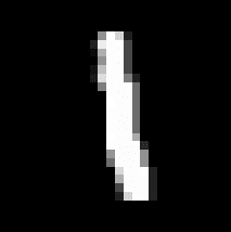
The challenges each provide a pre-trained network, and the task is to reverse engineer the network as well as to infer the labeling function used for training. The first challenge network is a MNIST CNN that takes MNIST images and outputs labels. The hints given are that [1] the labels are binary, [2] the test set accuracy is 95.58%, [3] that the (secret) labeling function is simple, and [4] this image:

The MNIST network consists of

• 2 Convolutional layers (Conv -> ReLU -> Dropout -> Pool)x2
• 2 Fully connected layers (fc1[400,200] -> ReLU -> fc2[200,2])

and we can access the data (torchvision.datasets.MNIST) but not the ground truth labels.

 

Spoilers ahead!

 

---

Summary of our solution (TL,DR)

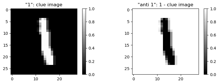
1. The inputs are labelled based on similarity with a 1 versus similarity with an inverted 1 ("anti-1"). If the difference is large (either clearly 1 or clearly anti-1) the image is labeled as class 0, otherwise the image is labeled as class 0. Specifically, the template for 1 seems to be is the given hint (clue_image), and the "anti-1" is 1-clue_image.
   
2. The similarity is measured as the sum over the element-wise product of the image matrices (or equivalently dot product of flattened image arrays).
   Then the the ~17k most similar images to “1” and ~14k most similar images to “anti 1” are labelled class 1, the remaining ~29k images are labelled class 0. We can also phrase this as a band filter for similarity with (clue_image - 0.5), defining class 0 as where -17305 < (image * (clue_image - 0.5)).sum() < -7762.
   We can observe this internally by looking at the embedding in the 200-neurons space, a PCA decomposition colored by label shows how the model judges this similarity:
   
3. The model internally implements this via two groups of feature detectors (in the 200-dimensional neuron layer). These are “1-detectors” (detecting clue_image) and “anti-1-detectors” (detecting 1-clue_image). If either group fires sufficiently strongly, the model is classified as class 1, otherwise class 0.
   
4. This classification has 96.2% overlap with model labels. Since the model itself has only 95.6% accuracy on the test set we think the difference is plausibly due to model error.
5. We test our hypothesis with Causal Scrubbing. Specifically we test our hypothesis that of the 200 neurons there are 48 neurons detecting "1" similarity, 31 neurons detecting "anti-1" similarity, and 121 dead (useless) neurons. We resample-ablate all neurons by replacing each neurons activation with its activation on a different dataset example where our hypothesis predicts it to have a similar activation.

Part 1: How we found this solution

Since the model prediction depends on the logit (final neuron) difference we can directly say that in the final layer we only care about the logit of label 1 minus the logit of label 0, the logit diff direction. Then, using the [200,2] fc2 weight matrix (biases irrelevant) we can directly translate this logit diff direction into the 200-dim neuron space (by taking the difference of the respective weight vectors). We will make use of the logit diff directions at multiple points throughout the analysis.

PCA decomposition

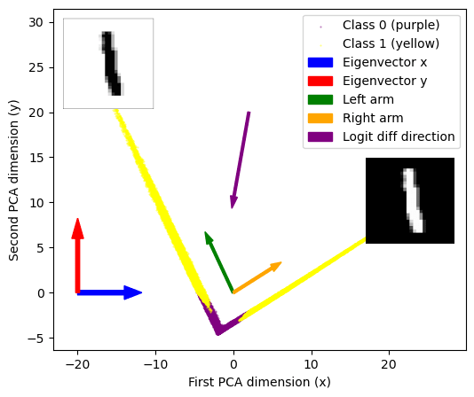
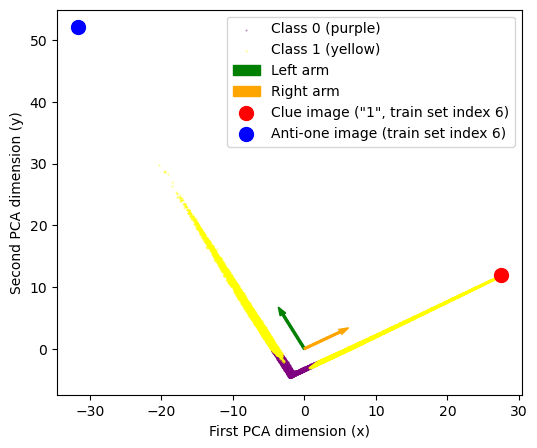
First we look at the 200-dim layer of neurons. Plotting a PCA decomposition of the activations at that layer into 2 dimensions (90-ish % variance explained) shows a striking V-shape i.e. all data points distributed along just two lines. Adding color=labels to the plot we see that all class 0-labelled data points lie in the bottom of the plot, at the corner of that V-shape.

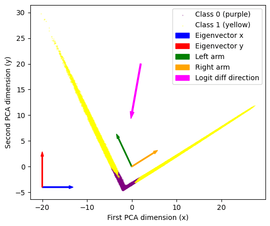
It looks like these embeddings basically contain the classification! We can read off that

• Eigenvector 0 describes where points are along the V-shape. We call the points at x<-2 the left “arm”, and the x>-2 part the right arm. Points near the corner (x ~ -2) are the ones classified as class 0.
• Eigenvector 1 describes how far points are away from the corner of the V-shape. So that low values along this direction correspond approximately to class 0, high labels to class 1.

Seeing the particular shape of this plot we know that we don't actually care about the PCA eigenvectors, but about these “arm-directions”, the two directions corresponding to the yellow arms. We can simply get those directions with a quick & dirty linear regression (we’ve added those to the PCA plot as arrows). Finally we can also add the logit diff direction (remember from above, this was a 200-dimensional vector) to the plot. As expected it just points downwards to the corner of the V.

Feature visualizations

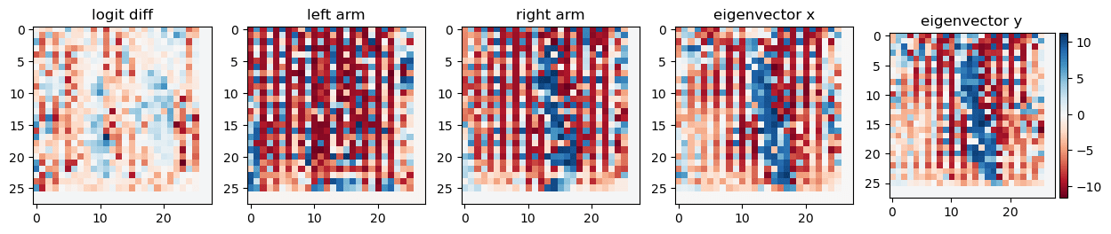
Now let us learn what all those directions mean. We initially computed feature visualizations by generating inputs that maximize the activation of a neuron/direction for the logit diff direction, the eigenvectors, and the arm-vectors without a super clear result:

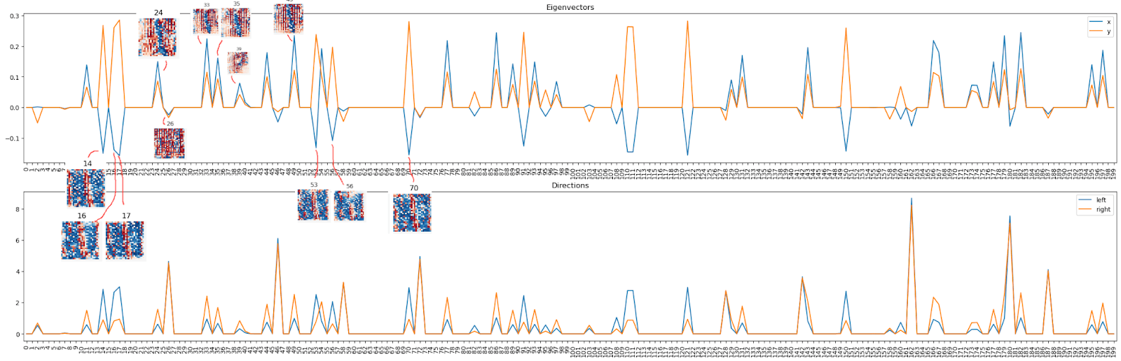
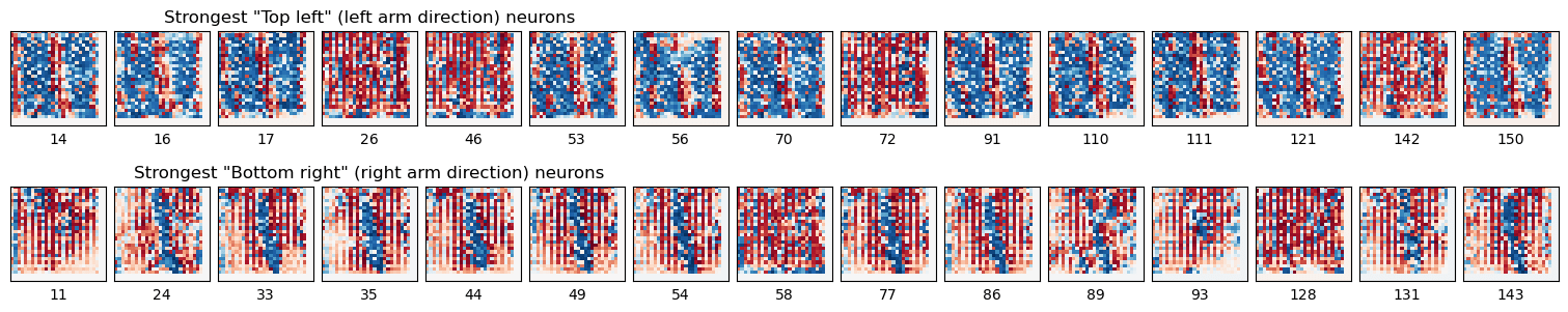
As a next step we compute the feature visualizations for all 200 neurons in this layer: We notice mostly two types of neurons: Positive and negative “1”-shapes, pointed out by red and blue arrows, respectively. Keep these neuron numbers in mind for the very next paragraph!

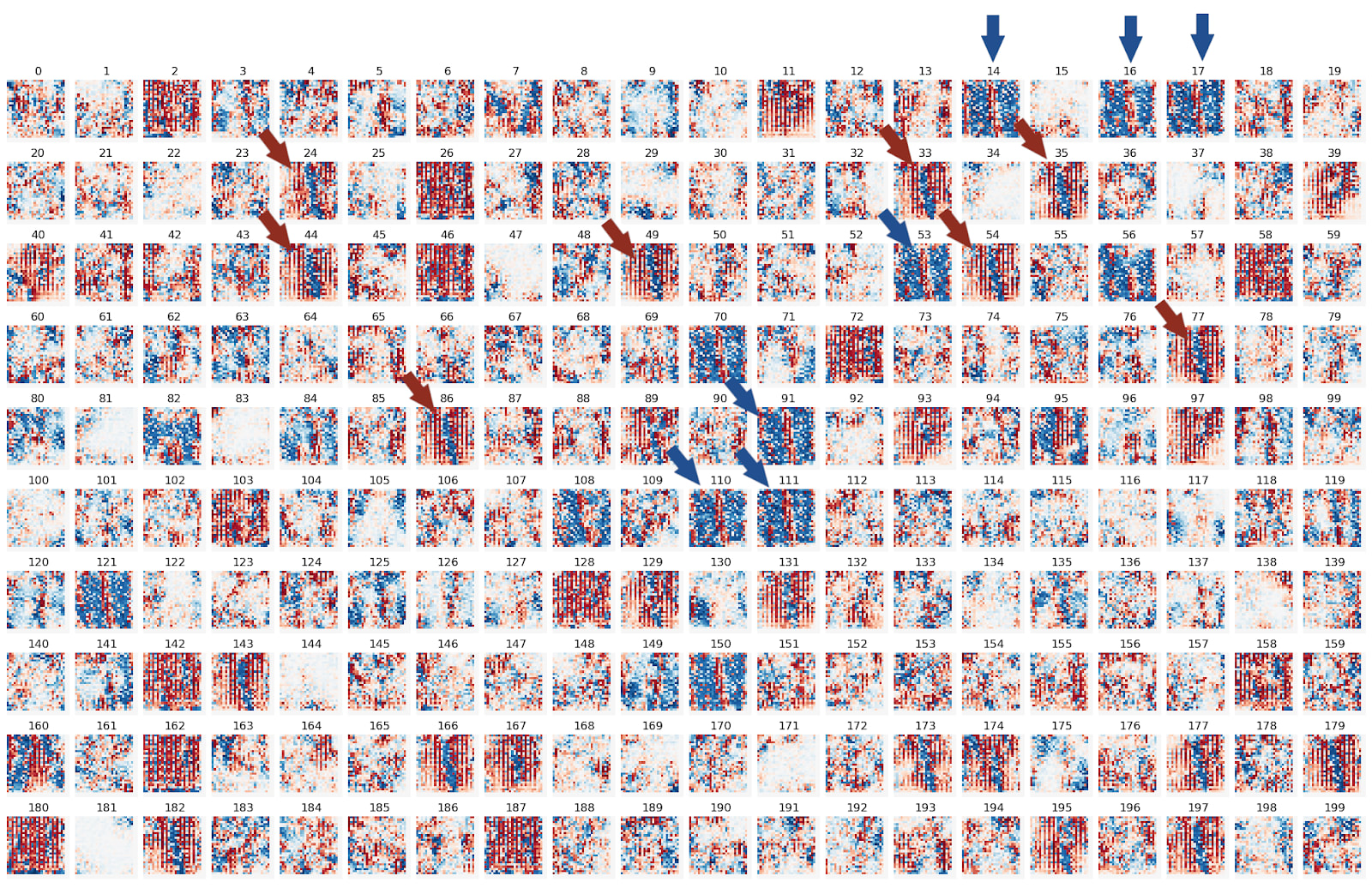
Now we look at the eigenvectors (top panel) or arm-vectors (the left & right arm in PCA plot, bottom panel) in this 200-dim space. We notice these vectors make use mostly of a couple of neurons only -- and these are the same neurons as we observed above!

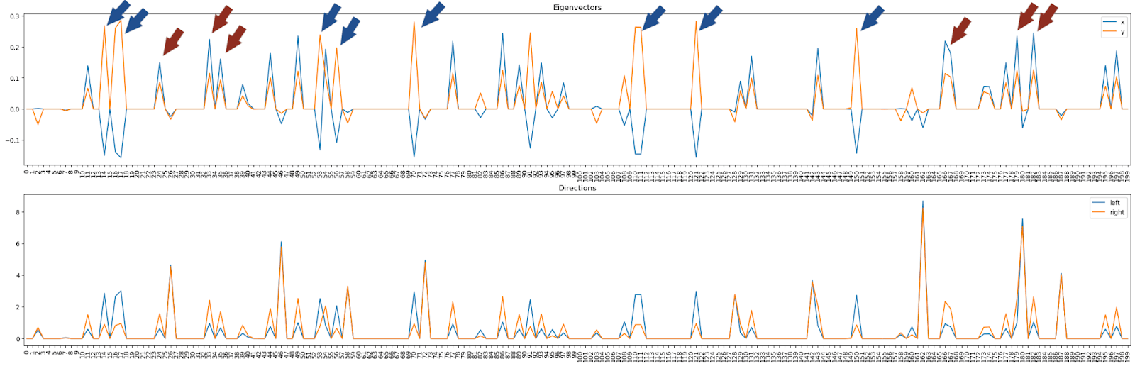
Looking at the top panel, we see some neurons activate both eigenvectors positively (we call them “top right direction neurons” since "both eigenvectors" points into the top right corner of the PCA image), and some neurons activate the first one (x) negatively and the second one (y) positively (“top left direction neurons”). These top left and top right directions correspond to the left- and right-arm directions as we confirm explicitly in the panel below (shows arm directions rather than PCA dimensions).

Interesting aside: Every neuron contributes towards positive logit diff direction, no neuron contributes the other way! We can make this clear by plotting the logit diff contribution for every neuron, weighted by their typical activation: The bottom row is always blue and the top row always red, i.e. all activate in a similar direction. This is atypical, usually you would expect neurons contributing to each class, but here any of the significant neurons firing contributes to class 1. This may be suggestive of "class 0 is just everything else".

Back to the eigenvectors / arm directions. We noticed there are two types of neurons, so let’s look at the corresponding visualizations and we notice Oh! All the “top right” ones (both positive) correspond to a sort of “1” (with some stripes), and all the “top left” ones correspond to a kinda “anti-1” (color map always as above, blue = positive, red = negative).

Here is a sorted list of the 15 strongest "top left" and "bottom right" neurons:

This gave us the idea that maybe we are detecting “1-ness” of images, so we put the clue image (dataset image number 6, which is a “1”) on the PCA plot (big red dot). Turns out is the furthest-out example in the top-right arm! The obvious follow-up (furthest-out image in left arm) didn’t lead anywhere (it was a “0”, index 22752).

But back in the feature visualizations and noticed the “top left” neuron images looking like anti-ones. So we eventually tried the image `1 - clue_image` (= anti-1) and it perfectly matches the “top left” direction! (big blue dot)

Finding a suitable labeling criterion

So now we have a pretty good guess of what the two directions represent and now we just need to figure out the precise labeling criterion. A bit of trial and error shows that the similarity of the input with “1” minus the similarity with “negative 1” = torch.ones(28,28) - clue_image matches the labels well. In particular we compare this in two ways

• Does the histogram of labels as a function of our proposed criterion look cleanly separable
• Does it seem that the first PCA direction (which does separate the classes) maps tightly to the proposed criterion (scatter plot)

The first way is closer to the challenge goal and gives us a binary signal per data point, while the second one is closer to what the network does and, importantly, gives us a continuous measure of how good the proposed criterion is so that we could try out different ideas and iterate. For similarity metric we eventually found the sum over the element-wise product of the matrices (i.e. the dot product of the flattened matrices). We compare this with  “clue_image - 0.5” which is equivalent to the difference found initially.

This plot shows our final solution (top), as well as a previous idea (bottom) for illustration of what we are looking for. The left side shows the histogram, and the right side shows the scatter plot, as explained above. The final solution (i) cleanly separates the classes, and (ii) shows a pretty tight relation to the PCA direction. Compare this to the (worse) lower panel to see what we were looking for.

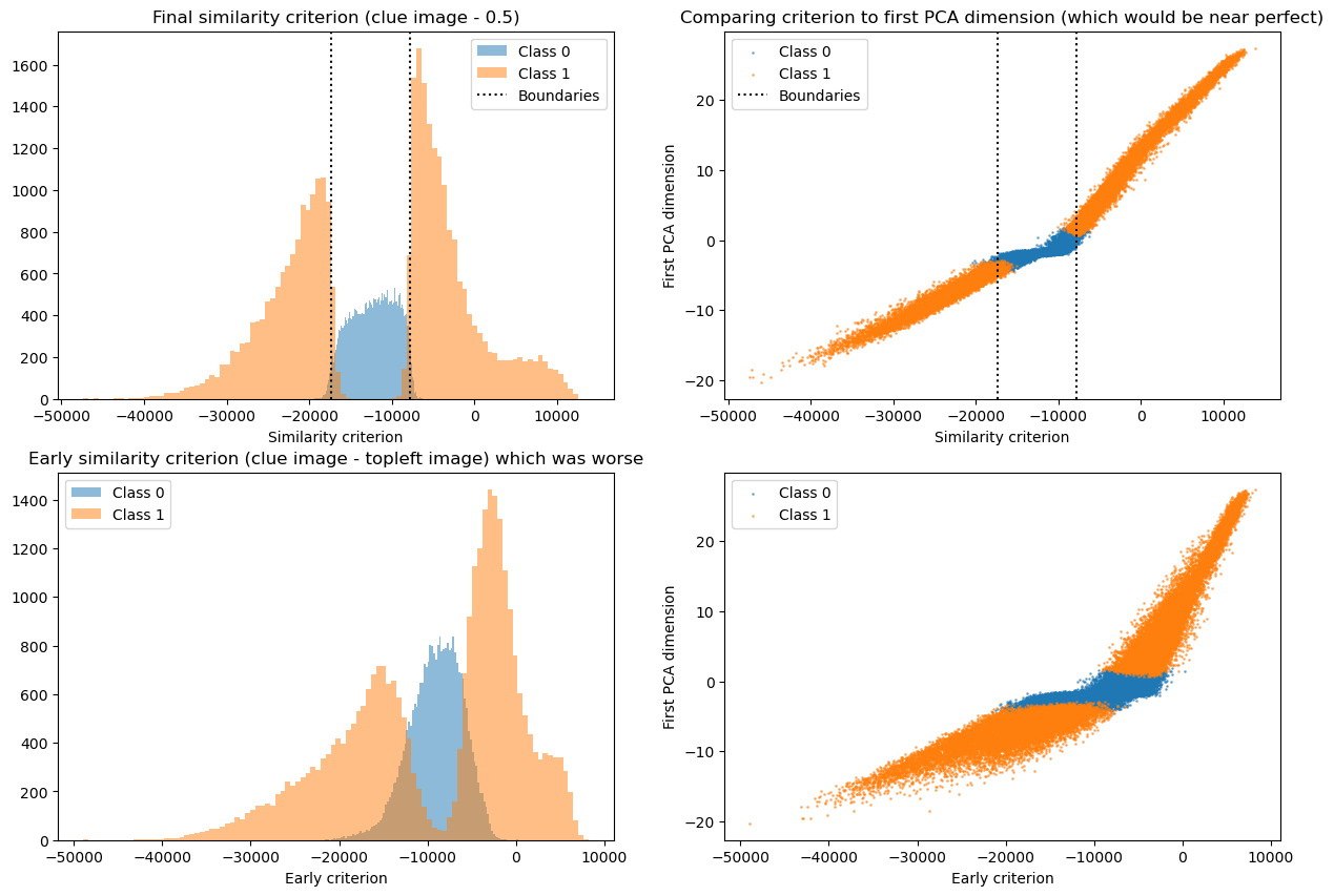
The labeling function -17305 < (image * (clue_image - 0.5)).sum() < -7762 (in words: dot product to [clue_image minus grey image]) recovers model performance with 96.2% accuracy (fraction of points classified identically to real model). Since the model itself only recovers ground truth accuracy with 95.6% we don’t necessarily expect there to be a better simple solution.

Internally this seems to be implemented as a bunch of neurons that detect 1 and anti-1 and assign samples to class 1 if sufficiently similar to 1 and anti-1, otherwise the default is class 0.

Part 2: Mechanistic evidence, interventions, and Causal Scrubbing

The above reasoning provides a strong hypothesis of what the network does. However, we want to test this hypothesis by intervening in the proposed mechanisms. 

Zero ablations and direct logit attribution

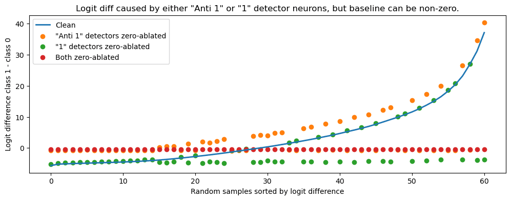
The first and obvious test is to ablate the “1” and “anti 1” detector neurons. You might expect zero-ablation to work (we did) since neurons only detect special patterns but this turned out to not work -- here we explain why: The baseline for the “anti 1” detectors is below zero, so that zero-ablating them raises almost all data points to class 1.

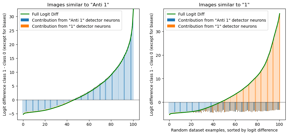
To see this we looked at a form of direct logit attribution, attributing the logit difference to the two groups of neurons. The figure below shows the logit difference effect (y-axis) of zero-ablating a set of detectors (colors) for some random input images (x-axis). Most images (x-axis) excite either the “1” detectors (green), “anti 1” detectors (orange), or neither (x-axis left side). This makes sense remembering the PCA plot from above, we recall that data points lie either along the left arm (starts to excite “anti 1”) or right arm (excite “1” detector), but not both.

To confirm this (and also test our similarity idea) we split the data set in two, according to our similarity score. Then we plot the logit difference in a stacked bar chart, as a sum of contributions from “1” detector and “anti 1” detector neurons. We see the pattern exactly as predicted, only one of the contributes in every category. (We also nicely see the negative baseline from the “anti 1” detector that caused our issues earlier.)

Minimum ablation interventions

Now that we are aware of the baseline behavior, and that there are two groups of neurons which each deal with “1”-similar or “anti 1”-similar images, we can ablate the neurons. We ablate a neuron by replacing its activation with its dataset-minimum. As we saw in the previous figure this represents the baseline for no detection.

The next figure shows this minimum-ablation. We split all neurons into two groups, the 31 “anti 1 detectors” and 48 “1 detectors”. We see (left panel) that ablating either reduces the logit difference, i.e. points less to class 1 (which contains the “1” and “anti 1” images) and more towards class 0.

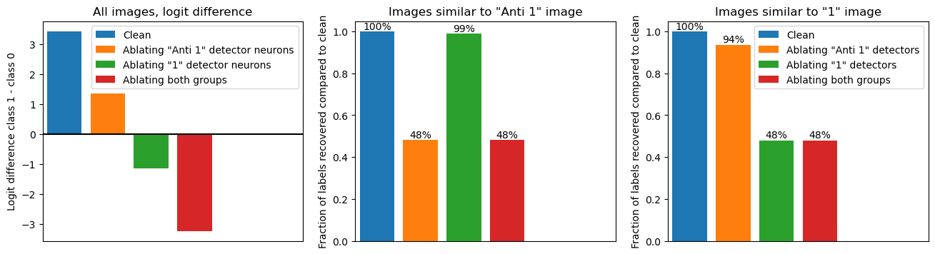
Furthermore, our classification of the detectors predicts that the first group should only be relevant for images that are more similar to the respective group, so we test this in the next two pane;s (middle and right, legend shown right only). We measure what fraction of the dataset labels is changed by the ablation of neurons in either group.

Amazingly, the results are exactly as expected! For images similar to the “anti 1” image (middle panel), ablating the “anti 1” detector (orange) reduces performance to random chance (50%), while ablating "1" detectors (green) has barely any effect. And equivalently, for images similar to the “1” image (left panel): Ablating "anti 1" detectors (orange) barely affects performance while ablating "1" detectors (green) reduces performance to random chance. As expected, ablating both (red) always destroys performance.

Causal Scrubbing

Finally we decide to apply the most rigorous test to our results by using the Causal Scrubbing framework to devise the maximum resampling-ablations allowed by our hypothesis.

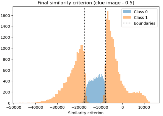
Concretely we have claimed that there exist “1” detector neurons, “anti 1” detector neurons, and "dead" (useless) neurons. Additionally we claim that our similarity criterion (dot product with “1” - 0.5 image) splits the data set into three parts as illustrated in the histogram below: The left part (activates “anti 1” detectors), the middle (activates neither), and the right part (activates “1” detectors).

  This would imply that

1. 1 detector neurons are active for images similar to "1" (right orange region) and inactive for otherwise (left and middle region)
2. Anti 1 detector neurons are active for images similar to "anti 1" (left orange region) and inactive for otherwise (left and middle region)
3. Useless neurons have no effect and are never active (left, middle, and right region)

and our hypothesis implies that these regions are defined by our similarity criterion. 

In our causal scrubbing experiment we test all of these predictions, randomly resampling all neurons within their permitted groups. Specifically

1. We resample any dead neurons with its activation on a random dataset example.
2. Any alleged “1” detector neurons we replace based on what our hypothesis claims:
   1. If it should be inactive (i.e. if input is in the left or middle region), we replace its activations with those from any random other image where it should be inactive, i.e. draw a random image from the left and middle region of the histogram.
   2. If it should be active (i.e. if input is in the right region) we replace its activations with those from a similar image, i.e. we select a random replacement that is within ~ 0.01% to 10% in similarity score.
3. Any alleged “anti 1” detector neurons we replace based equivalently.
   1. If it should be inactive (i.e. if input is in the right or middle region), we replace its activations with those from any random other image where it should be inactive, i.e. draw a random image from the right and middle region of the histogram.
   2. If it should be active (i.e. if input is in the left region) we replace its activations with those from a similar image, i.e. we select a random replacement that is within ~ 0.01% to 10% in similarity score.

Below we show how much accuracy is preserved while applying all these resample-ablations at the same time. Accuracy is measured as fraction of model labels that are unaffected by the resample ablations. The one variable is the notion of replacing images with another similar image, we scan a range of similarity thresholds from 0.01% deviation in similarity score (x-axis of histogram above) all the way to 10% (very different images). 

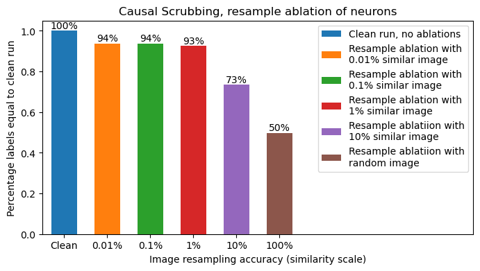
We find a very impressive 93% - 94% preserved performance for all reasonable similarity thresholds, only dropping below 93% when at >1% similarity threshold. The 94% performance is in line with what we saw in previous sections, showing ~6% of model behavior is not compatible with our hypothesis. This is a strong result for a Causal Scrubbing  test, and gives us confidence in the tested hypothesis.

Conclusion: We have solved this Mechanistic Interpretability challenge by understanding what the model does, and found the correct labeling function (confirmed by the challenge author who we sent a preview of this post). The most useful tool for understanding this network turned out to be PCA decomposition of the embeddings and feature visualizations, with the Causal Scrubbing and Intervention tests clarifying our understanding and correcting slight misconceptions. See the TL,DR section [LW · GW] at the top for the highlights of the post.

Acknowledgements: Many thanks to Esben Kran and Apart Research for organizing the Alignment Jam, and to Joe Hardie and Safe AI London for setting up our local hack site! Thank you to Stephen Casper for challenging us! Thanks to Kola Ayonrinde for pointing out the observations that all neurons cause positive logit difference! And thanks to the EA Cambridge crowd, in particular Dennis Akar and Bilal Chughtai, for helping Stefan wrestle PyTorch indexing!

1 comments

Comments sorted by top scores.