Solving the Mechanistic Interpretability challenges: EIS VII Challenge 2
post by StefanHex (Stefan42), Marius Hobbhahn (marius-hobbhahn) · 2023-05-25T15:37:54.593Z · LW · GW · 1 commentsContents
  Summary of our solution (TL,DR)
  Main investigation and evidence
    Task reasoning
    Model mostly works if we fix the attention pattern
    Task is already solved at resid_mid (basically)
    What the MLP does
    Understanding the residual stream
  Interventions, tests, and Causal Scrubbing
    Causal Scrubbing
  Conclusion
    Can we tell what the true labeling function is though?
    Stephen Casper's conclusion, after seeing our post
    Other approaches we tried / why do we focus on embeddings?
  Discussion on fixing attn pattern
  Appendix:
      PCA plots but colored by ground truth rather than model labels:
      PCA plot of the third and fourth dimension (we showed only first and second dimension in the post):
      MLP animations for fixed attention models:
None
1 comment
We solved* the second Mechanistic Interpretability challenge (Transformer) that Stephen Casper [AF · GW] posed in EIS VII [AF · GW]. We spent the last Alignment Jam hackathon attempting to solve the two challenges presented there, see here [AF · GW] for our solution to the first challenge (CNN). The challenges each provide a pre-trained network, and the task is to
- Find the labeling function that the network was trained with
- Find the mechanism by which the network works.
*We have understood the network’s labeling mechanism, but not found the original labeling function. Instead we have made a strong argument that it would be intractable to find the labeling function, as we claim that the network has not actually learned the labeling function.
A notebook reproducing all results in this post can be found here (requires no GPU, around ~10GB RAM).
Note that our solution descriptions are optimized with hindsight and skip all wrong paths and unnecessary techniques we tried. It took us, two somewhat experienced researchers, ~24 working hours to basically get the solutions for each challenge, and a couple days more for Stefan to perform the interventions, implement Causal Scrubbing tests, interventions & animations, and to write-up this post.
Task: The second challenge network is a 1-layer transformer consisting of embedding (W_E and W_pos), an Attention layer, and an MLP layer. There are no LayerNorms and neither the attention matrices nor the unembedding have biases.
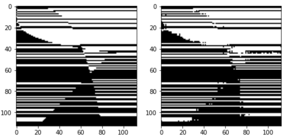
The transformer is trained on sequences [A, B, C] to predict the next token. A and B are integer tokens from a = 0 to 112, C is always the same token (113). The answer is always either the token 0 or 1. If we consider all inputs we get 113x113 combinations which we can shape into an image to get the image from the challenge (copied below). Black is token 0, and white is token 1. The left panel shows the ground truth, and the right panel the model labels. The model is 98.6% accurate on the full dataset.
Spoilers ahead!
Summary of our solution (TL,DR)
We found that the model basically just learns the shapes by heart, it does not learn any mathematical equations. Concretely we claim that
- The model barely uses the attention mechanism. Even if we fix the attention pattern to the dataset-mean, the model labels 92.7% of points correctly. We reverse-engineer the fixed-attention version of the transformer for simplicity, and we don’t expect any interesting mechanics in the attention mechanism but rather basically random noise the model has learned.
- With attention fixed, the post-attention residual stream (
resid_mid) at token C is just an "extended embedding", it is a linear combination of the token A and B embeddings. We show that the model classification can already be read off at this point.- In particular we claim that these extended embeddings are largely determined by a linear combination of two embedding directions.
- These directions correspond to input filters, this equivalence exists because we fixed the attention pattern and thus
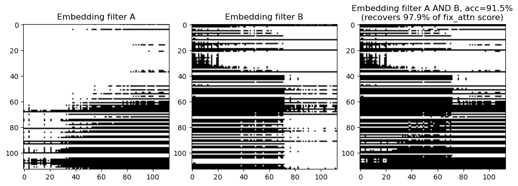
resid_midis given by a linear combination of the embeddings. - The classification is given by class 1 = Filter 1 AND Filter 2 (with some threshold numbers). We can illustrate this as binary mask using those thresholds: The left two images are filters learned by the model, and their AND-combination (3rd image) reproduces the model output to a large extent:
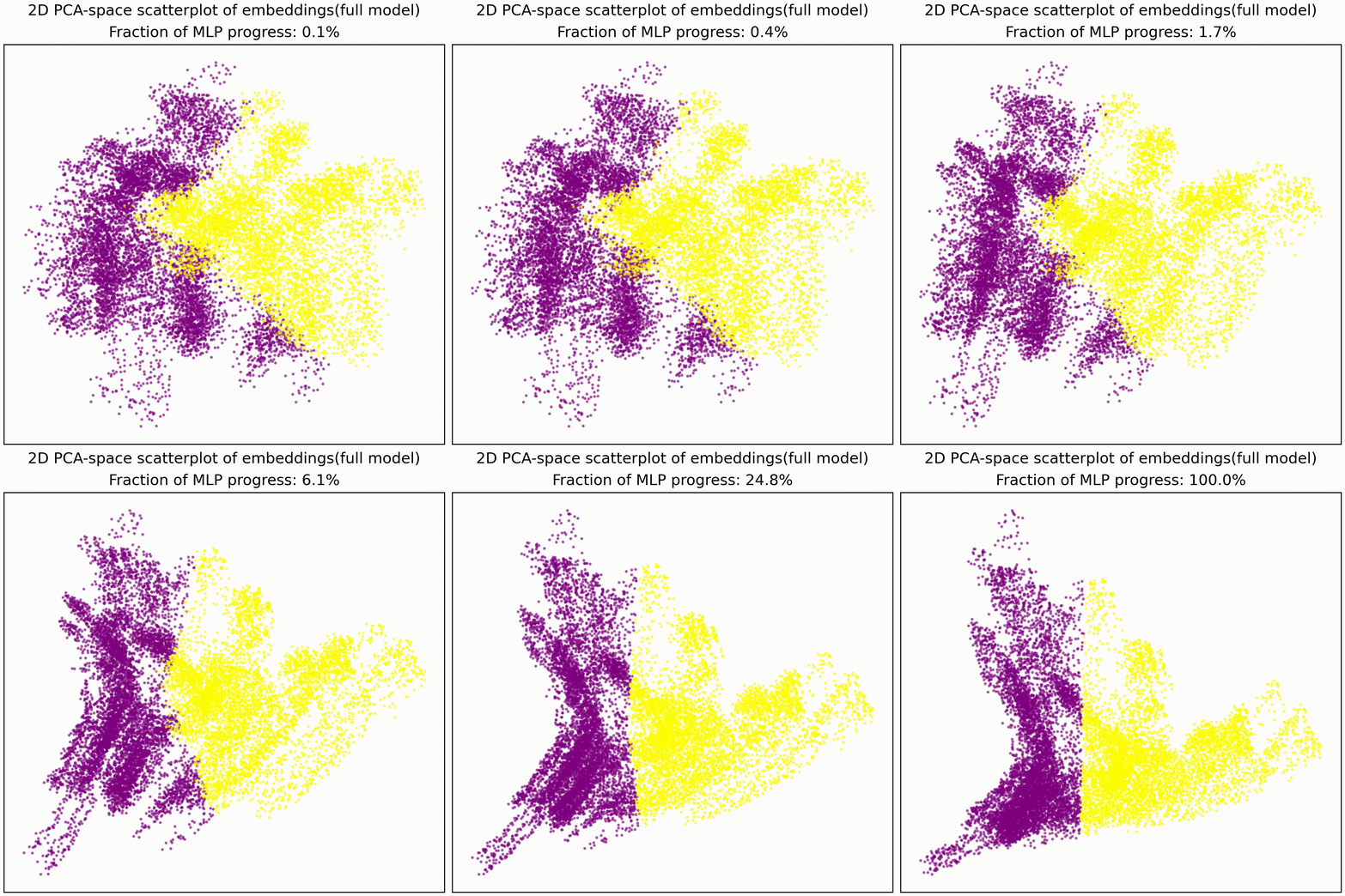
- The MLP basically just implements this AND gate, a simple non-linear transformation of the embedding into a linearly separable form. The animations below illustrates this:
- We test whether these PCA features we identified indeed correspond to the values of the two filters: If this hypothesis is true then randomly sampling data points to be equal on one filter, but random on the other filter, should give us a straight line in PCA space: It does.

- Causal Scrubbing & Interventions: We test the hypothesis that: The model performance is determined by the AND-combinations of the two identified filters only. This should allow a list of resampling ablations. We transform the 128-dim data into 128-dim PCA space (affine linear transformation, completely reversible), then perform resample-ablations in all 128 PCA dimensions. We measure performance as “fraction of labels identical to clean full model. We find that we recover 94% performance (full model) even under all possible resampling ablations.
Main investigation and evidence
Task reasoning
We don’t know whether the training loss included all positions or only the last token prediction, but in any case we only expect meaningful computation for the last position. If the model had to predict the other tokens, token B were just random, and token C would trivially always be 113, so only the final position output is interesting. Thus we focus on the residual stream at token position C.
Model mostly works if we fix the attention pattern
We first looked at the attention mechanism. We couldn’t see any obvious pattern in the attention behavior (QK circuits) so we tried to fix the attention pattern to constants, basically disabling the attention mechanism. We fixed each head’s attention pattern to the respective dataset-mean and found that the fixed-attention network gives the same answer as the full model in 92.9% of cases. (The full model achieves 98.6% correct labels on the data, while the fixed-attention model gives the correct label, compared to ground truth, in 92.7% of cases.)
This is a surprisingly large percentage and suggests that the attention mechanism does not play a large role in the model. A lot of our later analysis will focus on the fixed-attention model. We show both, the full and fixed-attention models in the following sections.
Note: Cas quotes the model’s test accuracy as 97.27%. We assumed in the post that Cas’ used a different convention to calculate the accuracy, after submitting we learned that Cas assumed the model to be 100% correct on the training set and thus 97.27% correct on the test set. In any case, in our write-up we never used this convention and always quote the full-dataset-accuracy (referred to as “correct-fraction”) since we do not have access to the training vs test split.
Task is already solved at resid_mid (basically)
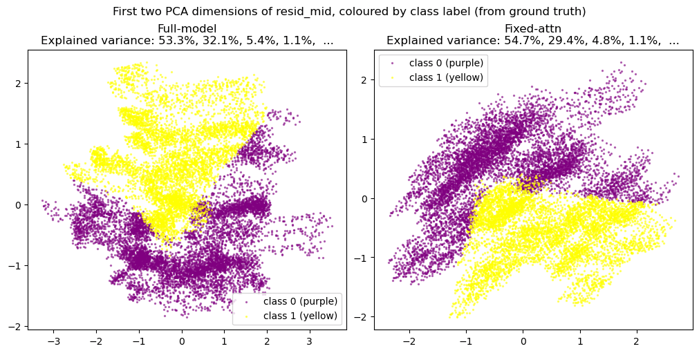
The embedding (resid_pre) at the final position (token C) is constant and trivial since the token is always the same (113). The important embeddings, coming from the previous two tokens, are added by the attention layer. So the post-attention residual stream (resid_mid) is the first non-trivial part of the residual stream. We apply a Principal Component Analysis (PCA) decomposition to resid_mid, and plot the first two components colored by the respective model labels (plots colored by ground truth, and plots of the next two PCA components, are given in the appendix).
We were very surprised to already see such a clear distinction between labels at this point!
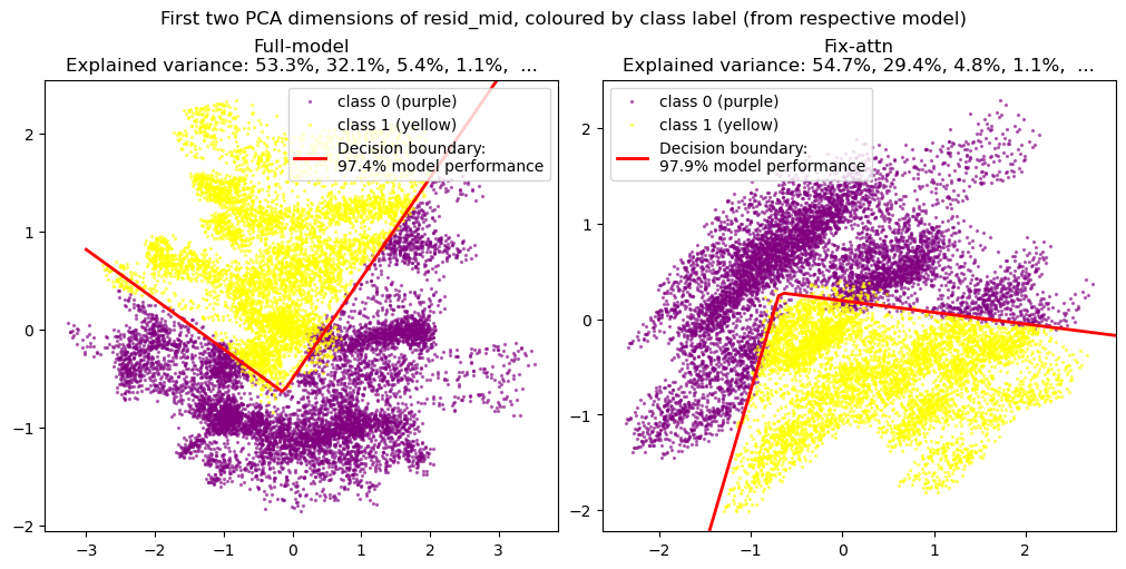
resid_mid shows the task is basically solved at resid_mid, for fixed-attention and full model.This implies that the task is largely solved at this point. The model clearly has sorted the inputs into class 0 and 1 categories; all that’s needed beyond this point is drawing the (quite simple) decision boundary.
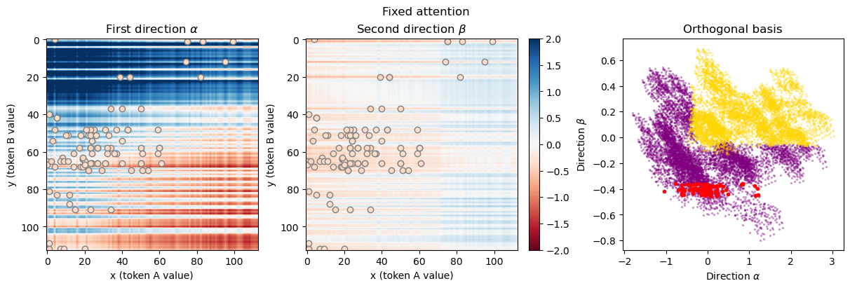
There are two clear directions that are relevant for the class separation (indicated with red lines), which correspond to two N-dimensional residual-stream directions that we call α and β (where N=128 is the embedding size). Using those vectors alone (red lines) we can recover 97.4% and 97.9% of the model performance for the full model and fixed-attention model (compared to their respective labels). Note that the classification is basically an AND-gate for class 1.
What the MLP does
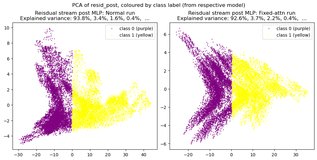
Applying a PCA fit to the post-MLP residual stream (resid_post) shows that, indeed, the MLPs transformed the previously non-linear decision boundary into a simple linear one that can be picked up by the unembedding.
We note that this is not particularly impressive for an MLP; the decision boundary was already pretty piecewise linear and this is a very-standard task for MLPs. This animation gives an intuition for what the MLP does, showing the residual stream (projected into resid_post PCA basis) for (i) adding 0..100% of the MLP output, or for (ii) adding the 1024 MLP neurons one by one. These animations are from the full model, the fixed-attention model looks similar (see appendix).
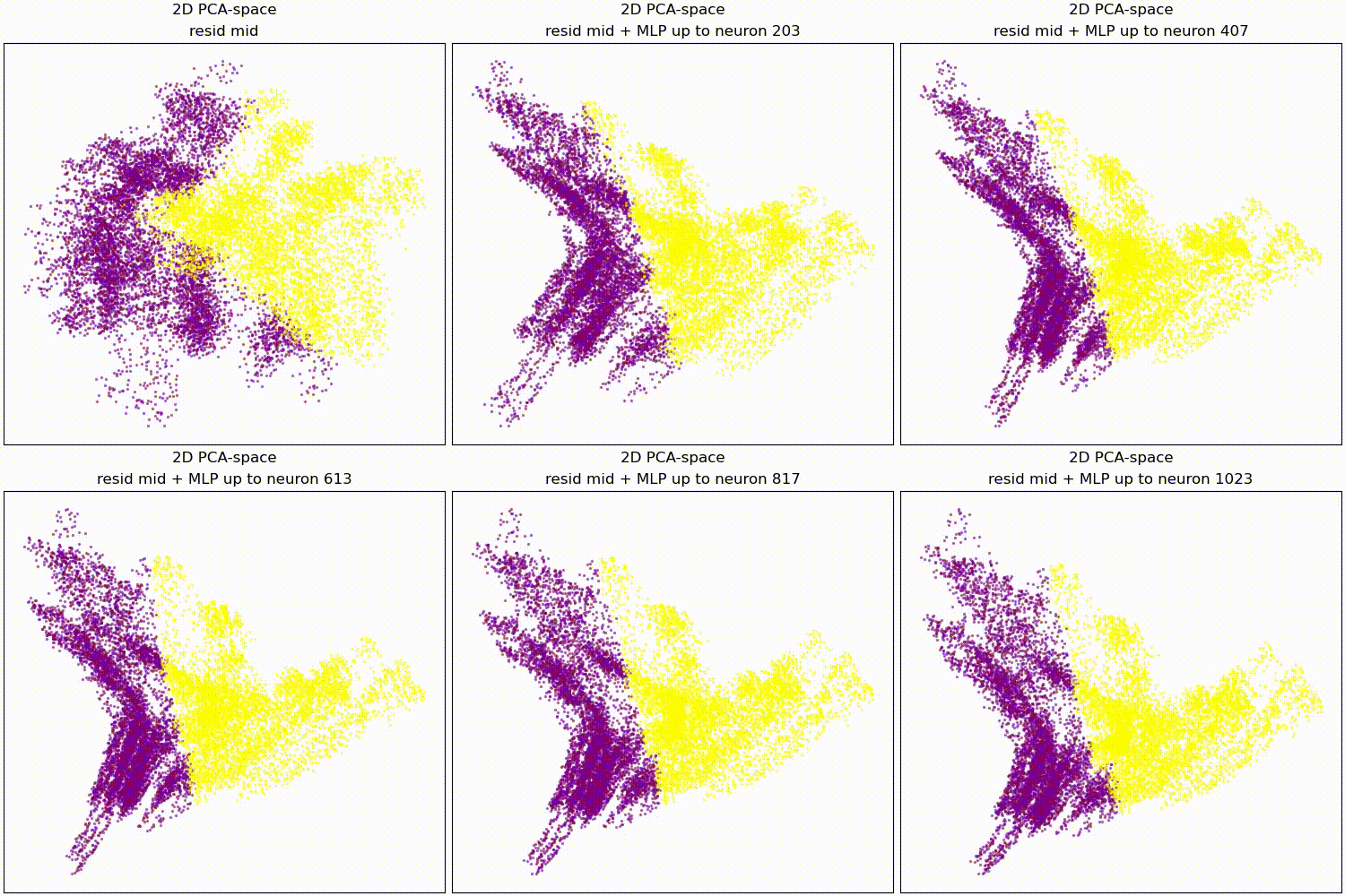
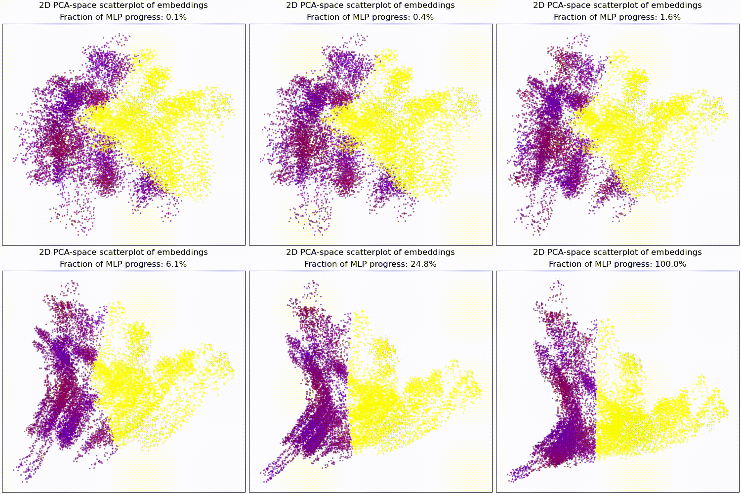
mlp_out from 0% to 100%.Understanding the residual stream
So far we have seen that the interesting part of the task is already solved at resid_mid, and that the MLPs appear to do nothing advanced. We also have seen that fixing the attention pattern barely influences the model behavior, so from here on we will analyze the fixed-attention model only.
This gives us the opportunity to Anthropic-style fully decompose the -dimensional residual stream at resid_mid into individual embedding terms: The residual stream resid_mid, as a function of the inputs and (one-hot vectors corresponding to the first and second input token) is
where and are combinations of the embedding matrix and the attention OV-circuit matrices and . In particular gives us 8 embedding matrices (one per attention head), and the above matrices are given by a sum over attention heads, weighted with the mean attention of each head pays to source position A or B
and (equivalently defined) are dimensional matrices ( is the vocab size) describe everything that goes into resid_mid.
And we can reduce this even further! We know from before than basically just two residual stream directions matter, α and β ( dimensional vectors). So we can reduce each dimensional matrix into two -dimensional vectors telling us how much or being a certain number pushes us into the α or β direction. The vector consists of 114 numbers, telling us how much resid_mid moves into direction if is that number. We display the raw vectors here, with the 114 dimensions on the horizontal axis (full version below, but hard to read). Don't worry, we will show more human-friendly visualizations below!
And we can see some basic features. For example, in the last row (see the full plot below, look at i.e. the effect of the -variable on the β direction), you can see that lower values contribute negatively and larger values positively – thus the β-filter approximately makes large values more likely to be class 1:
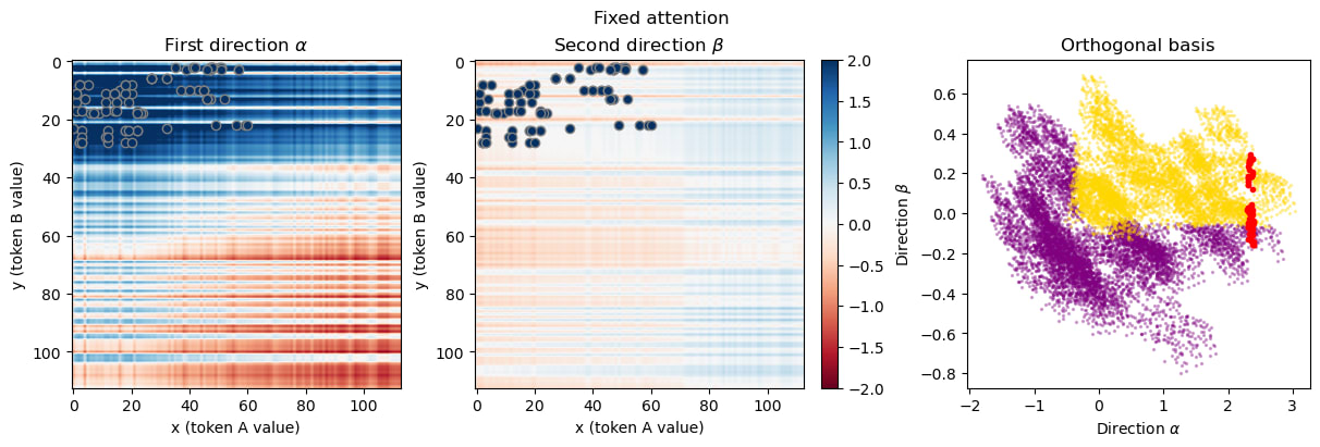
To make this visualization a bit more intuitive, we can combine the two -dim vectors for α and β into one low-rank matrix each. The intuition here is that the two α vectors both contribute additively to the α-filter (based on x and y variables respectively), so the matrix shows the α-direction value for any pair of inputs:
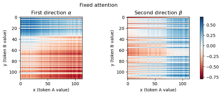
So these matrices tell us directly about the α- and β-direction values for every input. But we have said that the model performance is basically an α and β filter, with known thresholds (derived from fitting decision boundaries to the resid_mid PCA-transformed embeddings). We we can apply these thresholds here and show the resulting binary α and β filters below (first and second panel):
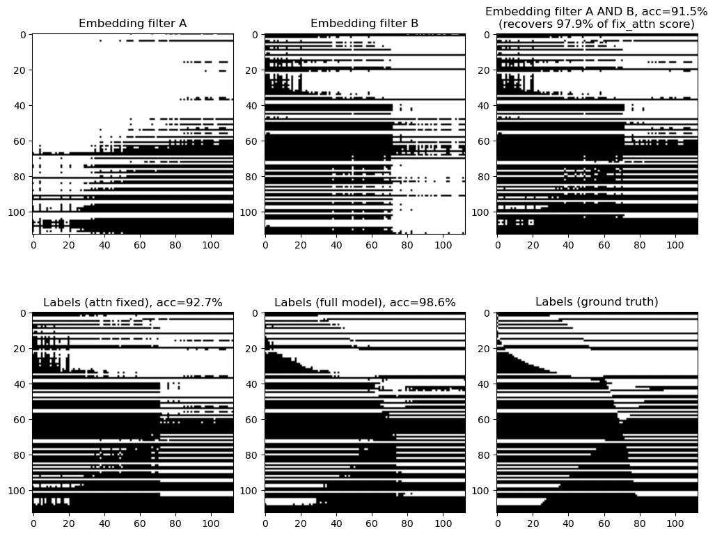
Then we can also show α AND β (third panel) and confirm, the AND gate is 97.9% identical with the output of the fixed-attention model (fourth panel). This is presumably below 100% due to us using only the first two PCA dimensions – using more dimensions would give us additional filters.
These results (third panel) do not fully (91.5%) overlap with the full model (5th panel) because we did not take the attention into account, so that our resid_mid embeddings are slightly different. The MLP being basically an AND gate applies to the full model as well though, as we saw in Figure 1, where the decision boundary fit recovered 97.4% performance.
Interventions, tests, and Causal Scrubbing
Here are two claims we want to briefly test: (1) We understand the step from resid_mid to outputs, understanding what the MLPs do. (2) We understand the step from inputs to resid_mid, understanding how the relevant resid_mid directions are derived from the inputs.
(1) Since we claim to understand the residual stream, we should be able to predict what happens when we add a random vector to it. We predict that the model label continues to be predicted by the PCA-projected decision boundaries as shown in Figure 1.
As a first test we add some random 128-dim vectors to the embedding (resid_mid in fixed-attention model) and re-compute the model labels. We use the original PCA projection and decision boundaries, to observe whether this still correctly predict the labels, i.e. does a point crossing the red boundary correspond it changing it color? The animations show two different random vectors, scaled from length 0 to 10:
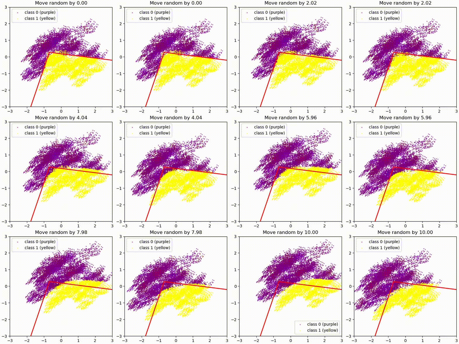
We also run the same test shifting along the decision boundary vectors, rather than random vectors.
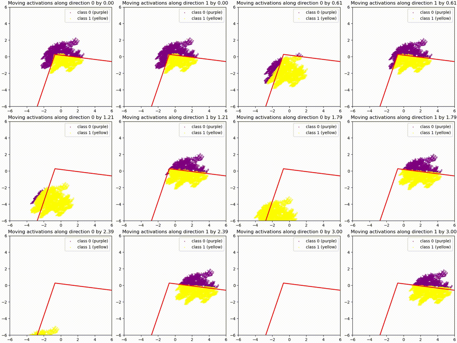
In both cases we see that the prediction holds for small changes, but breaks down quickly for large changes. This seems reasonable given that all of these tests pass out-of-distribution activations to the network, and the MLP is not actually an AND gate between two PCA directions but only approximates it.
(2) Our other claim was that these PCA dimensions are directly given by the α and β filters we present above. This would predict that, if we pick data points with the same color value on one of the filters, they appear as a line parallel to this filter’s decision boundary in the PCA plot. We test this for a couple of random colors here (picked to illustrate different colors but not cherry-picked, random examples look like this too):
This works exactly as expected, when the points fall on the same α-filter value (left panel) they lie on the same α-direction (x-axis value in right panel), and vice versa.
Causal Scrubbing
We formulate our hypothesis to test it in the causal scrubbing [AF · GW] framework: We claim that the model output depends only on two filters (α and β residual stream directions) with binary outputs, and specifically is given by the logical AND between the two filters. (This tests the part from resid_mid to outputs, not the first part tested above -- we could include that too but by resample-ablating by filter-image color rather than filter-direction value but we did not try this.)
We can test this hypothesis by performing all resampling-ablations that should be allowed by our claim. Specifically we decompose this into the following claims with corresponding resample-ablations:
- Only 2 (or 3*) dimensions matter
→ [1] Resample-ablate all other 126 residual stream directions.
[1*] We also test resample-ablating all but the first three directions to check if we lost much by ignoring the 3rd direction. - Only whether the value is > or < the threshold matters in these 2 dimensions
→ [2] Resample ablate values on each side of the threshold, i.e. replace every dim-0 value with a random other dim-0 value that is one the same side of the threshold. - The output is the logical AND of 1st and 2nd direction > respective threshold:
→[3a] Resample-ablate dim-0 irrespective of dim-0 value where β (dim-1) is FALSE
→[3b] Resample-ablate dim-1 irrespective of dim-1 value where α (dim-0) is FALSE
To clarify the last points, consider the AND-gate of Filter α & Filter β: In this context we can see intervention [2] as "swap TRUE with TRUE and FALSE with FALSE". Then there is one more degree of freedom, swapping TRUE with FALSE as long as both are paired with a FALSE, which is represented by resampling ablations [3a] and [3b].
| FALSE & FALSE | FALSE & TRUE |
| TRUE & FALSE | TRUE & TRUE |
We apply all these ablations individually and together, and check how much performance is lost.[1]
Causal Scrubbing result for the fixed-attention model (performance measured with respect to ground truth, i.e. 92.9% is the maximum):
| Resampling: | 1 | 1* | 1+2 | 1+3a | 1+3b | 1+2+3a | 1+2+3b | 1+2+3a+3b |
| Performance: | 91.2% | 92.6% | 89.1% | 91.1% | 91% | 89.0% | 89.3% | 88.8% |
Causal Scrubbing result for full model (w.r.t. ground truth, expect 98.6% as the maximum):
| Resampling: | 1 | 1* | 1+2 | 1+3a | 1+3b | 1+2+3a | 1+2+3b | 1+2+3a+3b |
| Performance: | 97.1% | 99.3% | 94.1% | 96.6% | 96.2% | 94.0% | 94.4% | 94.1% |
The hypothesis is well compatible with the both models, we loose only around 4% performance in both cases. Eyeballing the numbers we think about 1-2% seem to come from using 2 rather than 3 PCA dimensions (resampling [1] vs [1*]), and another 2-3% seem to come from treating the filters as binary (resampling [2]).
In all cases these are strong results that support our hypothesis.
Conclusion
Our investigation has shown how the model performs (most of) this task internally. A large part of the model performance is achieved by memorizing the input data in a compressed fashion, fitting at least 91.5% of the data into just four 114-dimensional vectors / two rank-1 114x114 matrices.
We have reverse-engineered the fixed-attention model to a large degree (limited only by having chosen to ignore further PCA directions), and don’t expect interesting behavior in the attention QK-circuit of the full model.
Can we tell what the true labeling function is though?
Regarding the original labeling function, we cannot really read this off the weights because it appears the model mostly memorized the training data and interpolated to correctly label most of the test data. We wouldn’t see this as a loss for mechanistic interpretability: We could figure out what (most of) the model was doing, which is what we are actually interested in.
We don’t expect the original labeling function will improve our predictions for the model behavior.
Stephen Casper's conclusion, after seeing our post
I agree with this not being a loss in general for mechanistic interpretability. But this seems to be a counterexample to some of the reasons that people are optimistic about mechanistic interpretability.
I think that streetlighting and cherrypicking in mechanistic interpretability has led to a harmful notion that deep down, under the hood, neural networks are doing program induction. The main point of these challenges has been to see if and how simple mechanistic interpretability problems could be solved when the researchers did not get to hand pick the problem to study. I think this attempt at the challenge has been more than satisfactorily interesting and successful. I am enthusiastic about declaring this challenge solved (with an asterisk).
But not being able to recover the labelling function is still a limitation. To the extent that neural networks do interpolation instead of program induction (which there is a lot of theoretical and empirical support for), then we should not be looking for the type of thing that the progress measures paper showed. I think it is important to remember that Grokking -- thus far -- has only been demonstrated in toy contexts and has not shown to be useful for analyzing networks in the wild. This limitation also seems to dampen optimism about "microscope AI." Even if one has an excellent mechanistic understanding of a model, it may not transfer to useful domain knowledge.
My one critique of this solution is that I would have liked to see an understanding of why the transformer only seems to make mistakes near the parts of the domain where there are curved boundaries between regimes (see fig above with the colored curves). Meanwhile, the network did a great job of learning the periodic part of the solution that led to irregularly-spaced horizontal bars. Understanding why this is the case seems interesting but remains unsolved.
Other approaches we tried / why do we focus on embeddings?
In this write-up It looks like we immediately jumped to focusing on the embeddings and their decomposition, and did not consider any other techniques. This is because we only present the methods that were useful in the end. We tried a variety of other methods first and only identified the solution after trial and error; we investigated attention patterns and the QK circuits, attention result patching, MLP neuron ablation, and more, before we identified the structure in the embeddings.
Discussion on fixing attn pattern
We want to discuss why we mostly focus on the fixed attention model here. We can very thoroughly reverse-engineer the embeddings in the fixed attention model, and many findings hold approximately for the full model. And the causal scrubbing tests designed based on the explanation of the fixed attention model also work on the full model, proving that the second part of our explanation (that is tested by Causal Scrubbing) is very similar in the full model.
We expect to learn nothing interesting in the attention mechanism. Our hypothesis here is the following:
The varying attention changes the mixing between pos A and pos B embeddings, slightly perturbing the embeddings. The full model has learned to correct for this, it has just memorized the perturbed embeddings rather than the mean-attn embeddings we can visualize. There is probably no inherent advantage to having a more varied attn pattern, and a model trained with this fixed attn pattern could probably solve the task almost equally well. From the viewpoint of the fixed-attn model, these embedding perturbations look like noise that slightly throws-off the classification near the decision boundaries, possibly explaining where our explanation doesn't work well.
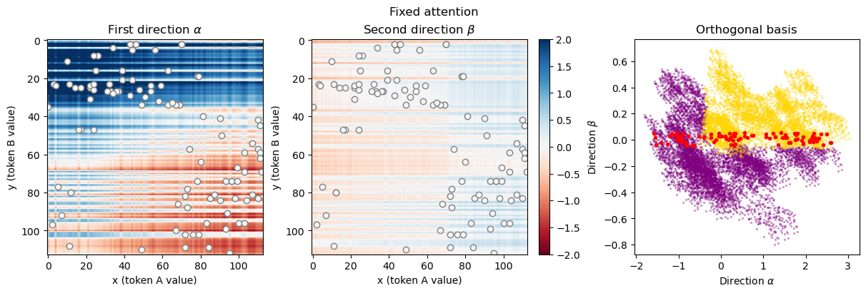
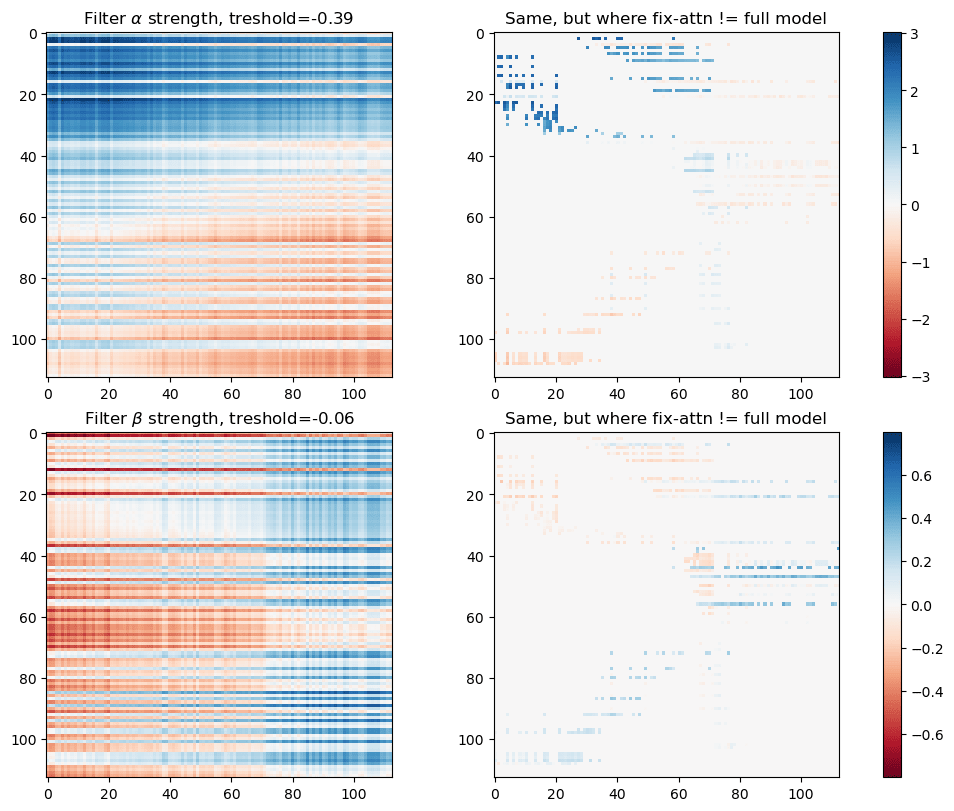
One prediction from this hypothesis: The points where the fix-attn model is wrong should correspond to filter-strengths near the threshold of at least one of the two filters.
Here is a plot of the filters (left, as shown before), and the filter values of misclassified points (right). The color scale in each row is the same; we can see the bottom and right points are near the threshold of filter α, and the points in the top left are near the threshold of filter β, as predicted!
This does not conclusively prove our hypothesis, but it looks pretty much as expected. So we are somewhat confident about the hypothesis and don’t think it’s worth spending more time on the attention mechanism.
For anyone interesting in investigating this though, we propose as a first step to view the full attention pattern as a perturbation of the mean pattern, i.e. attn = mean_attn + x*(attn-mean_attn), and approximating the effect of x on the result for small x. Here is an animation of the resid_mid PCA transformation while scaling x from 0 to 1:
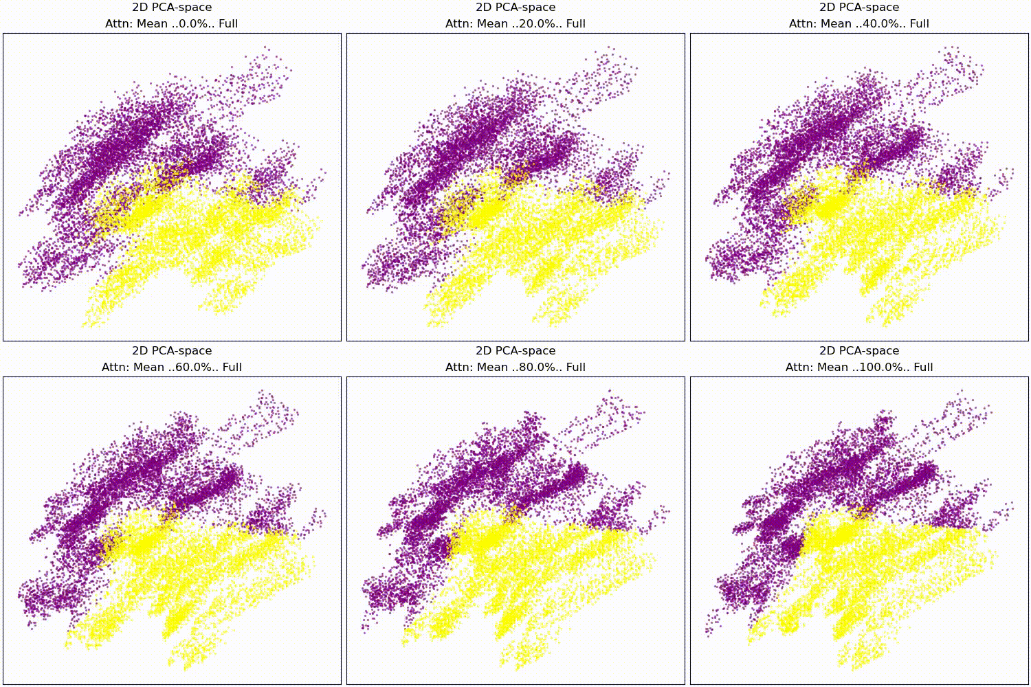
resid_mid embedding while scaling attention from dataset mean to full individual attention patterns.Appendix:
PCA plots but colored by ground truth rather than model labels:
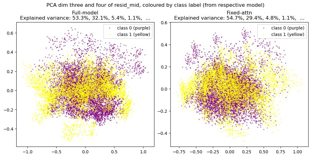
PCA plot of the third and fourth dimension (we showed only first and second dimension in the post):
MLP animations for fixed attention models:
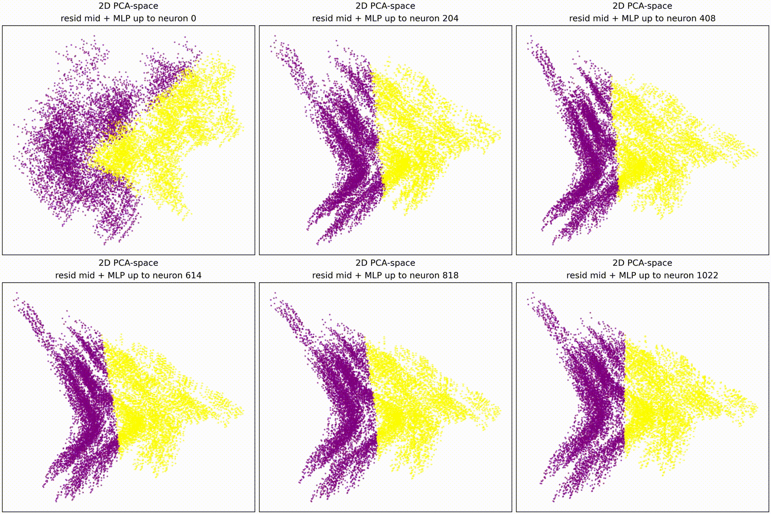
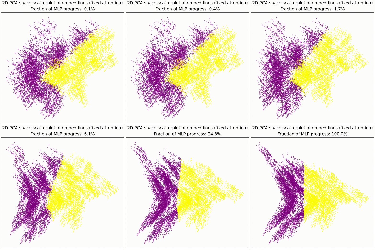
mlp_out from 0% to 100%.- ^
Implementation note: You can apply 1+2+3a or 1+2+3b with the pre-computed filter values, but if you apply 3b after 3a (or vice versa) you need to recompute filter values since 3 changes TRUE/FALSE values!
1 comments
Comments sorted by top scores.
