Investigating Sensitive Directions in GPT-2: An Improved Baseline and Comparative Analysis of SAEs
post by Daniel Lee (daniel-lee), StefanHex (Stefan42) · 2024-09-06T02:28:41.954Z · LW · GW · 0 commentsContents
  TL;DR
  Introduction
  Experiments and Results
    Experimental Overview
    Developing a Better Baseline
      Why the Difference Between Two Activations?
      Comparing Different Baselines
      Revisiting Pathological Errors Under New Baselines
    Comparative Analysis of SAEs
      SAE Reconstruction Error Extrapolation
      SAE Feature Extrapolation
  Conclusion
        Future Work:
  Appendix
    L2 Version of the Main Figures
    Supplementary Figures
None
No comments
Experiments and write-up by Daniel, with advice from Stefan. Github repo for the work can be found here.
Update (October 31, 2024): Our paper is now available on arXiv.
TL;DR
By perturbing activations along specific directions and measuring the resulting changes in the model output, we attempt to infer how much the directions matter for the model's computation. Through the sensitive directions experiments, we show that:
- Heimersheim (2024) [LW · GW]’s sensitive direction baselines (experiments 2 and 3) were flawed in that the perturbation direction involved subtracting the original activation. We propose an improved baseline direction (called cov-random mixture) which does not use the original activation.
- Gurnee (2024) [LW · GW]’s KL-div for SAE reconstruction errors no longer seems pathologically high when we use this improved baseline. However, there remains some variability across layers.
- We extend the sensitive direction experiments to perturbations into SAE feature directions, and find:
- SAE directions have smaller or greater impact on the model output than our cov-random mixture baseline, depending on the SAE type and L0.
- Lower L0 SAE feature directions have a greater impact on the model output.
- Feature directions from end-to-end SAEs do not exhibit a greater influence on the model output compared to those from traditional SAEs.
Introduction
One of the primary goals of mechanistic interpretability is to identify the abstractions that a model uses in its computation. Recently, several works have sought to understand these abstractions by observing how much the probabilities for next token prediction change when activations are perturbed along specific directions – a technique we’ll refer to as sensitive direction analysis. Heimersheim (2024) [LW · GW] demonstrated, for example, that perturbing from one real activation towards another real activation changes the model output earlier (shorter perturbation lengths) than perturbations into random directions. This finding supports the hypothesis that perturbations along true feature [LW(p) · GW(p)] directions have a greater impact on model outputs compared to other directions, motivated (Mendel 2024 [LW(p) · GW(p)]) by toy models of computation in superposition (Hänni 2024).
Several works have used sensitive direction analysis to analyze Sparse Autoencoders (SAEs). Perturbations along the SAE feature directions appear to alter the model output more significantly than random directions, suggesting that SAEs successfully uncover important “levers” used by the model (Lindsey 2024). However, SAE-reconstructed activation vectors also alter the model output much more than random perturbations of the same L2 distance from the base activation, an observation that puzzled the interpretability community (Gurnee 2024 [LW · GW]). This phenomenon was characterized as a pathological behavior of SAE reconstruction errors.
In this post, we expand on the work of Heimersheim (2024) [LW · GW], Gurnee (2024) [LW · GW], and Lindsey (2024) by further exploring different perturbation directions.
Experiments and Results
Experimental Overview
The experiments described in this report focus on perturbing an activation within the residual stream of GPT2-small. Specifically, we perform perturbation as follows:
where represents the original activation, α is the perturbation length, and d is the unit direction vector. To assess the impact on the model's output, we use two metrics: the KL divergence of the next token prediction probabilities (more specifically, KL(original prediction | prediction with substitution)) and the L2 distance from the original activation in the Layer 11 resid_post activations. The main figure uses KL, and the analogous figure with the L2 metric can be found in the appendix. We include L2 distance at Layer 11 because it exhibits more predictable behavior than KL. For example, we noticed that L2 distance at Layer 11 is linearly related to perturbation length when the length is small. Unless if otherwise stated, the perturbations are applied in Layer 6 resid_pre. Layer 6 was chosen because Braun 2024’s main results focus on end-to-end SAEs on Layer 6 activations.
The experiments are performed on approximately 2 million tokens (16,000 sequences, each with a length of 128). We perturb activations for all token positions. When we extrapolate the perturbation vector, we extend the vector from length 0 to 101 (for context, the mean L2 distance between two actual activations in Layer 6 resid_pre is 81.59). Our results mainly focus on the resulting curves of KL vs perturbation length or L2 distance at Layer 11 vs perturbation length.
We use the mean of KL or mean of L2 across the 2 million tokens as our main measure. Although using the mean makes it challenging to capture the individual shape of the KL or L2 curves for each perturbation directions, an important characteristic as noted in the activation plateaus discussed by Heimersheim 2024 [LW · GW], we use the mean under the assumption that directions with greater functional importance will, on average, induce a more significant change in the model's output.
Developing a Better Baseline
Lindsey 2024 and Gurnee 2024 [LW · GW] use random isotropic perturbation as their baseline. Both papers point out that this might be problematic because actual activations are not isotropic, and some sensitivity differences may be explained by that effect. Previous work by Heimersheim 2024 [LW · GW] attempts to address this issue by adjusting the mean and covariance matrix of the randomly generated activations to match real activations. However, the post's perturbation directions use the direction from the original activation toward another random activation (), which includes the negative of the original activation () as a component. This makes it an unfair comparison to directions that do not include the original activation[1]. Therefore, we propose two new baselines (cov-random mixture and real mixture) where the directions do not include the original activation.
Following is the list of perturbation directions discussed in this section:
- Isotropic random: Perturb into a random direction (no subtraction)
- Cov-random difference: Perturb along , i.e. from base towards a cov-random activation. This direction was used in Heimersheim 2024 [LW · GW] ("random direction").
- Cov-random mixture: Perturb along , i.e. into the difference of two randomly generated covariance matrix adjusted activations. This is the first new baseline proposed. This direction no longer contains the original activation.
- Real difference: Perturb along , i.e. from base towards another real activation. A real activation is sampled from the activations from ~2 million tokens. This direction was used in Heimersheim 2024 [LW · GW] ("random other"). Like the "cov-random difference", this direction contains the original activation.
- Real mixture: Perturb along , i.e. into the difference of two real activations (not the original activation). The real activations are sampled from the activations from ~2 million tokens. This is the second new baseline proposed. Like the "cov-random mixture", the real mixture no longer contains the original activation.
Why the Difference Between Two Activations?
Under the Linear Representation Hypothesis (LRH), we can represent an activation as
where is the activation of (hypothetical) feature i, is the unit “direction” vector of feature i, and b is the bias.
If we take the difference between two activations and , we get:
Therefore, assuming LRH, subtracting any two real activations is a linear combination of (hypothetical) true features without the bias term. We note that this will also include “negative features,” which is not expected to be as meaningful in the models.
Comparing Different Baselines
On average, perturbation directions that include the negative original activation () cause a greater change in the model output compared to those that do not include the original activation. In Figure 1, KL for "cov-random difference" is greater than KL for "cov-random mixture" and the KL for "real difference" is greater than KL for "real mixture." The trend holds for perturbations in Layer 2, though the difference is minimal when considering the L2 distance in Layer 11 metric (Supplementary Figure 1). This finding suggests that the "difference" directions may primarily reflect the subtraction of the original activation, which seems related to Lindsey 2024’s observation that “feature ablation” has a much greater effect than other perturbations including “feature doubling.” The result supports the use of "mixture" baselines to ensure a fair comparison with directions like SAE features or SAE errors, which do not necessarily involve the original activation.
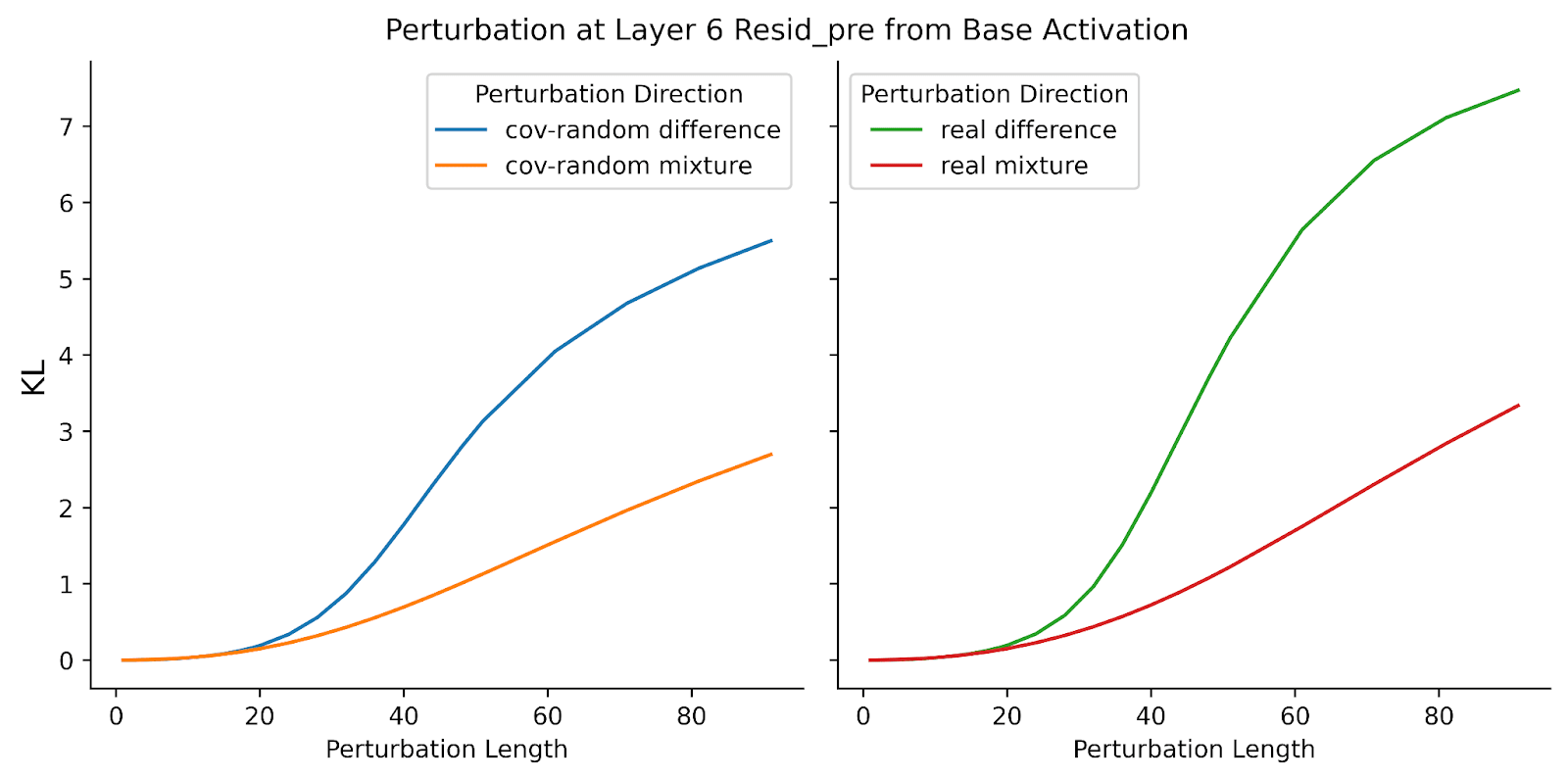
resid_pre. The x-axis is the perturbation length and the y-axis is the mean KL of logits. For the plot in the left column, we compare “cov-random difference” and “cov-random mixture.” For the plot in the right column, we compare “real difference” and “real mixture.” For both cases, the “difference” perturbations have a greater change in model output than “mixture” perturbations."Cov-random mixture" directions influence the model's output more significantly than isotropic random directions (right plot of Figure 2). This supports the hypothesis that isotropy reduces the impact of perturbations on the model’s logits. Since "cov-random" directions are derived from a multimodal normal distribution, and real activations are likely more clustered than normally distributed, we don’t expect "cov-random" directions to be the ideal baseline. Therefore, Heimersheim 2024 [LW · GW]'s finding that "real difference" directions altered the model’s output more dramatically than "cov-random difference" directions (replicated in the left plot of Figure 2) was unsurprising. However, the differences between "real mixture" and "cov-random mixture" directions are minimal, indicating that Heimersheim 2024 [LW · GW]’s result was influenced by the negative original activation component. A potential reason for the small difference between "cov-random mixture" and "real mixture" is that the former contains negative feature directions, which we don't expect to be meaningful.
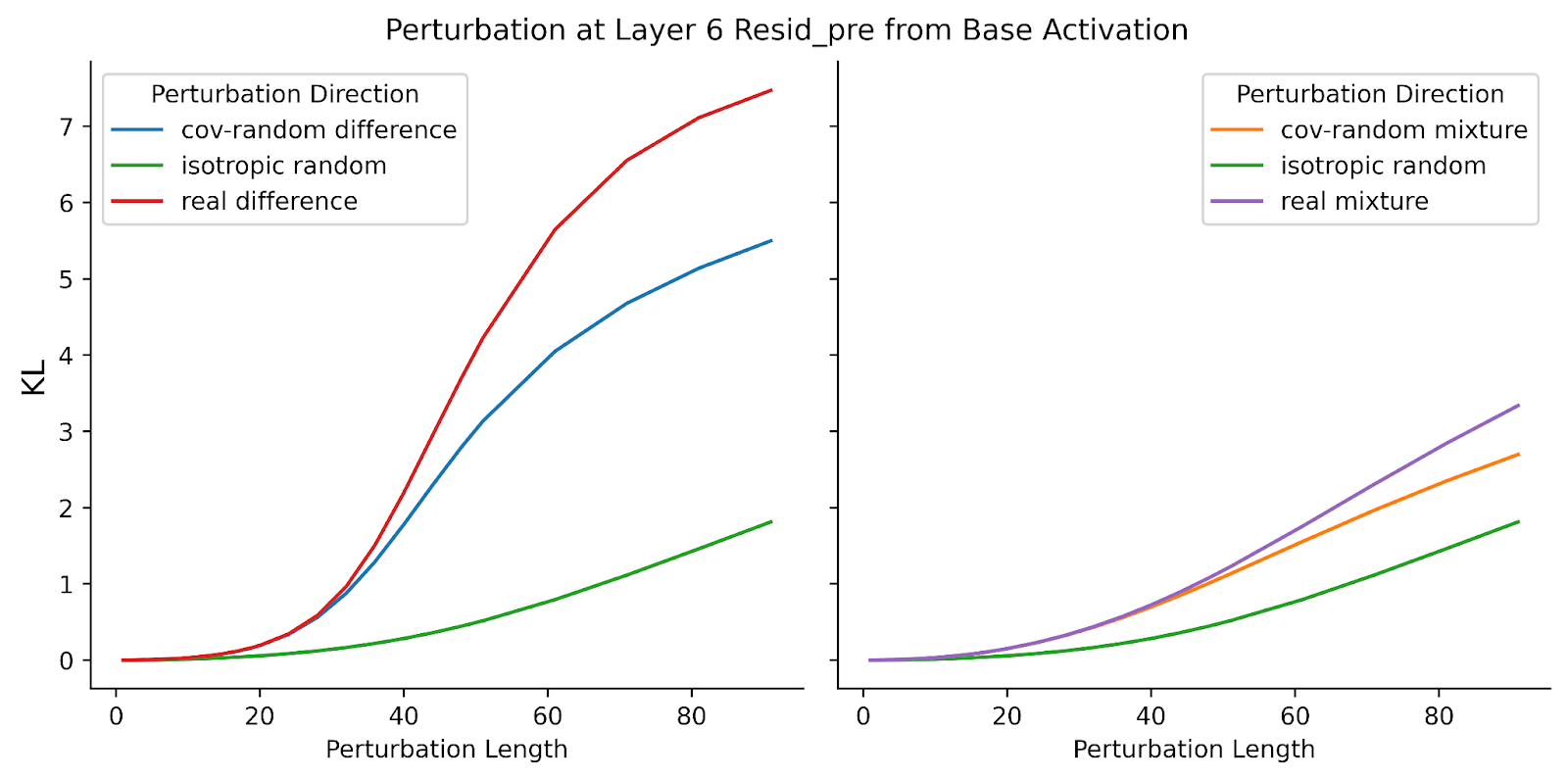
resid_pre. The x-axis is the perturbation length and the y-axis is the mean KL of logits . On the right, we compare “isotropic difference,” “cov-random difference,” and “real mixture.” On the left, we compare “isotropic random,” “cov-random mixture,” and “real mixture.” “Cov-random mixture” induces a significantly greater change in model output than isotropic random. While the model is more sensitive to “real mixture” directions than the two other perturbation types, there is minimal difference between “real mixture” and “cov-random mixture.”Revisiting Pathological Errors Under New Baselines
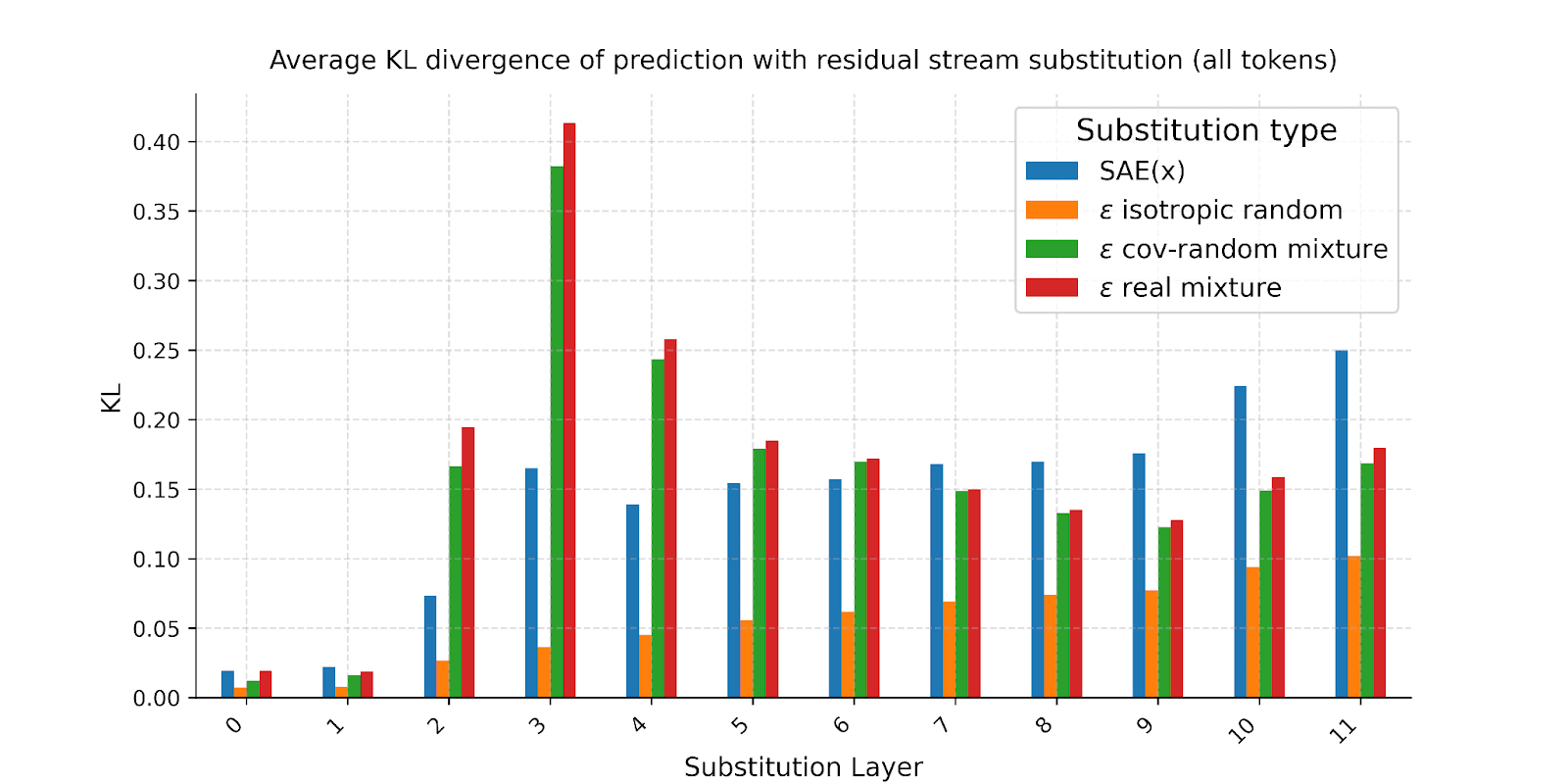
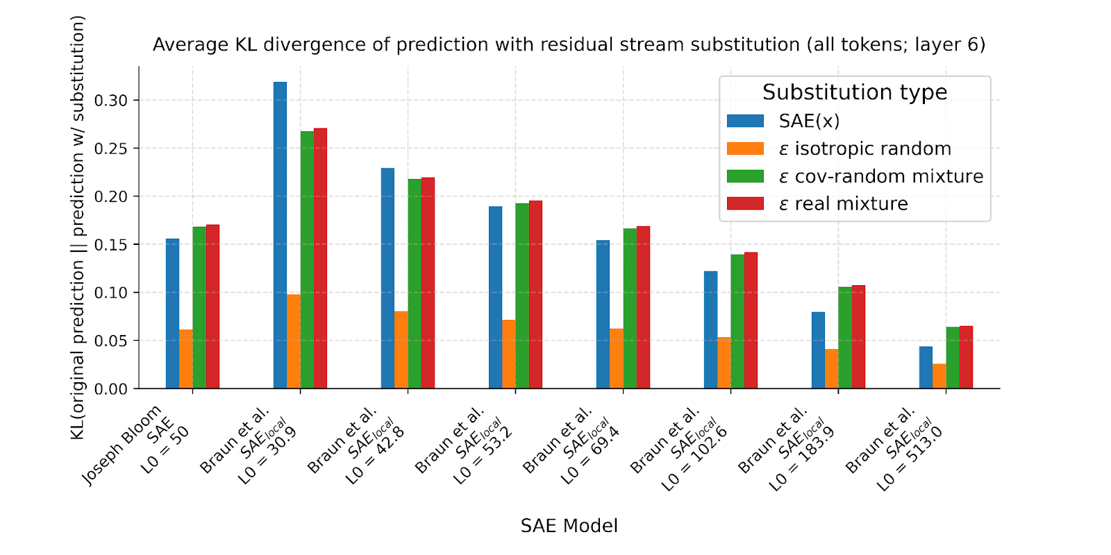
We reran the analysis from Gurnee 2024 [LW · GW], this time incorporating the two new baselines. We also compared multiple SAEs with different L0 values. Our results confirmed the original finding that substituting the base activation with the SAE reconstruction, SAE(x), changes the next token prediction probabilities significantly more than substituting an isotropically random point at the same distance (Figure 3). When perturbing along the cov-random mixture or real mixture directions, the average KL divergence is generally closer to that of SAE(x). However, there is considerable variability depending on the layer. For Layer 6, the SAE models across L0 generally seem to have nearly the same KL as that of cov-random mixture (Figure 4). While this suggests that addressing isotropy mitigates the previously observed pathologically high-KL behavior in SAE errors, questions remain about the variability observed across different layers.
Comparative Analysis of SAEs
Recently, a new type of SAEs called end-to-end SAEs has been introduced (Braun 2024). End-to-end SAEs aim to identify functionally important features by minimizing the KL divergence between the output logits of the original activations and those of the SAE-reconstructed activations. There are two variants of end-to-end SAEs: e2e SAE and e2e+ds SAE (where ds is short for downstream). Braun 2024 proposed e2e+ds SAEs as a superior approach because it also minimizes reconstruction errors in subsequent layers (whereas e2e SAEs might follow a different computational path through the network). In this section, we will compare traditional SAEs (or local SAE), e2e SAE, and e2e+ds SAE across various L0s.
Following is the list of perturbation directions discussed in this section:
- SAE Reconstruction Error Direction: Perturb along , i.e. from base activation towards the reconstructed activation.
- SAE Feature Direction: Perturb along , i.e. along one of the vectors i from the SAE dictionary. We choose SAE features that are alive, but not active in the given sequence.
SAE Reconstruction Error Extrapolation
To gain insight into the model sensitivity to SAE reconstruction errors, we extrapolate the error directions across various perturbation lengths.
We make the following observations and respective interpretations:
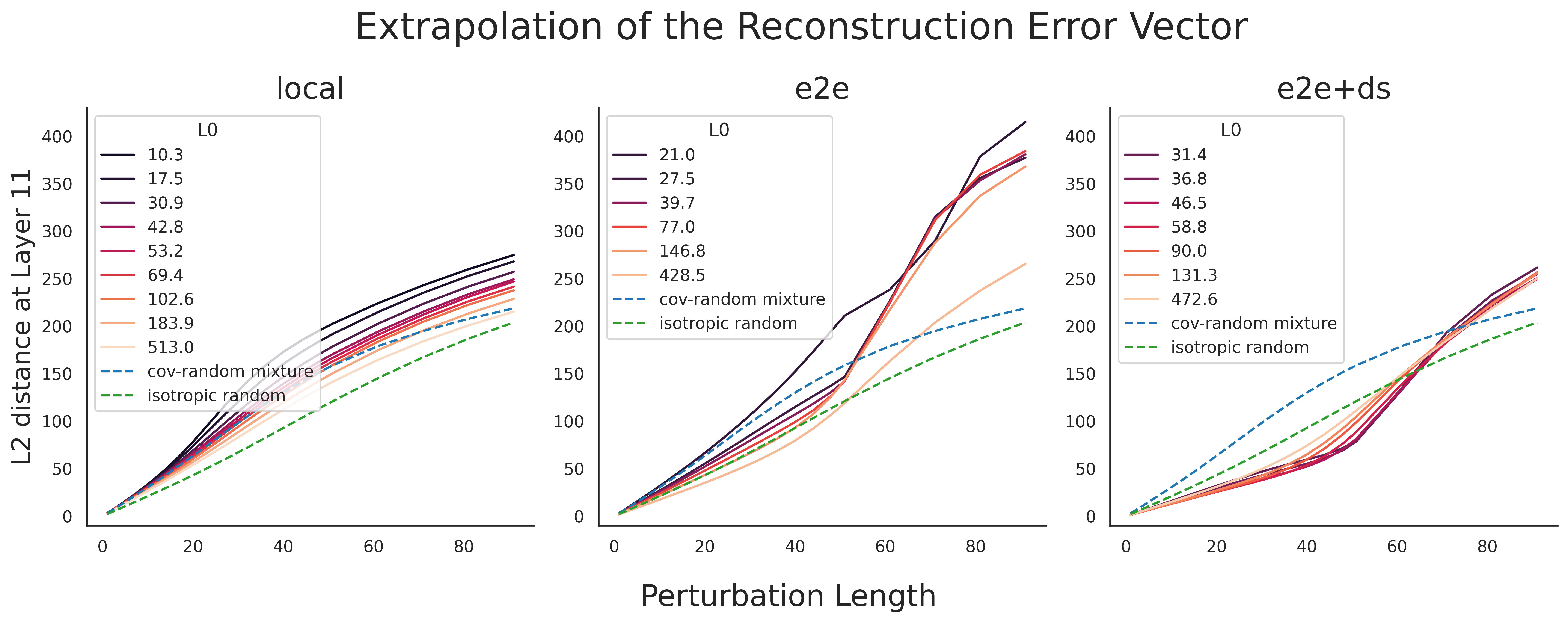
- For local SAEs, the behavior is straightforward: lower L0 corresponds to a stronger perturbation effect (left plot in Figure 5). For e2e (and e2e+ds) SAEs, the behavior is more complex: the effect of L0 at small perturbation scales is the opposite of its effect at larger scales. For perturbation lengths below ~50, lower L0 results in greater KL divergence for e2e and e2e+ds SAEs, except for L0 = 21.0 or 27.5 e2e SAEs (middle and right plots in Figure 6). For perturbations above 70, lower L0 corresponds to a stronger perturbation effect (Figure 5). This inversion of the L0 pattern disappears for e2e SAEs when we examine the L2 distance in Layer 11 (middle plot in L2 Figure 6).
- For reference, as noted earlier, the average L2 distance between two actual activations in Layer 6 resid_pre is 81.
- Since the L0 inversion disappears for L2 distance for e2e SAEs, we suspect the inversion is caused by the KL-minimizing training objectives of the end-to-end SAEs.
- While the curves for the local SAEs are close to the curves for the cov-random baseline, the curves deviate a lot for e2e and e2e+ds SAEs. Notably, the curves for e2e and e2e+ds SAEs remain low and then spike up from perturbation length of around 50 (Figure 5).
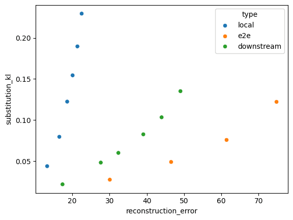
- The former is expected as e2e SAEs generally have a high L2 reconstruction error while having a low KL-divergence (Supplementary Figure 3).
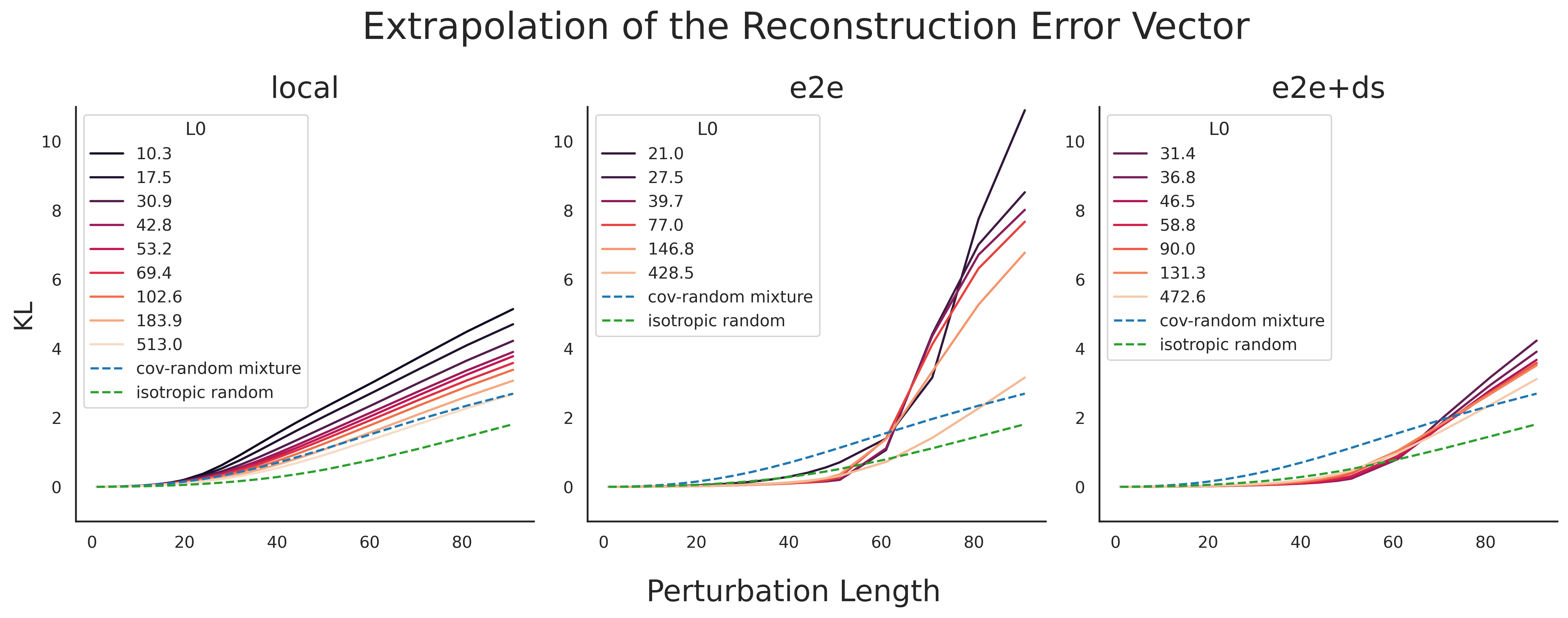
resid_pre. The x-axis is the perturbation length and the y-axis is the mean KL of logits. For the three columns, we compare the three different SAE model types. We compare the SAE reconstruction error directions with cov-random mixture and isotropic random directions. We color the lines by different L0 values of the SAEs.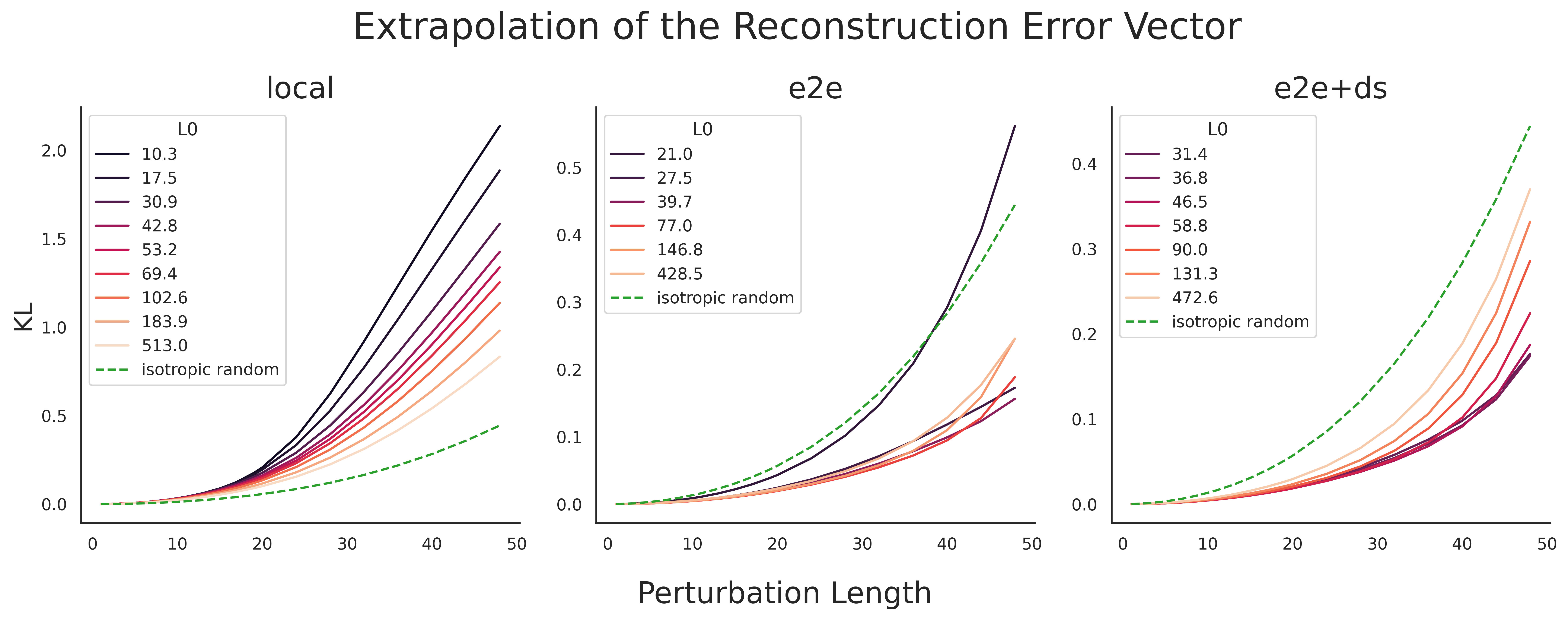
resid_pre. The x-axis is the perturbation length and the y-axis is the mean KL of logits. For the three columns, we compare the three different SAE model types. We compare the SAE reconstruction error directions with isotropic random directions. We color the lines by different L0 values of the SAEs. Note that the y-axis limit is not the same for the three plots.SAE Feature Extrapolation
To explore the functional relevance of SAE features, we extrapolate the SAE feature directions across various perturbation lengths. We select a random SAE feature that is alive, but not active in the given context the token is located in.
We make the following observations and respective interpretations:
- All SAE features have a greater impact on the model output than isotropic random directions (Figure 7). When compared to cov-random mixture, the effect varies based on the type of SAE and its L0 value.
- For all three types of SAEs, lower L0 corresponds to greater change in model output (Figure 7). For SAE features that are active in the given context (not shown here) we generally observed the same pattern.
- On the other hand, lower L0 SAE directions could just be more aligned with the higher principle components of the activation space.
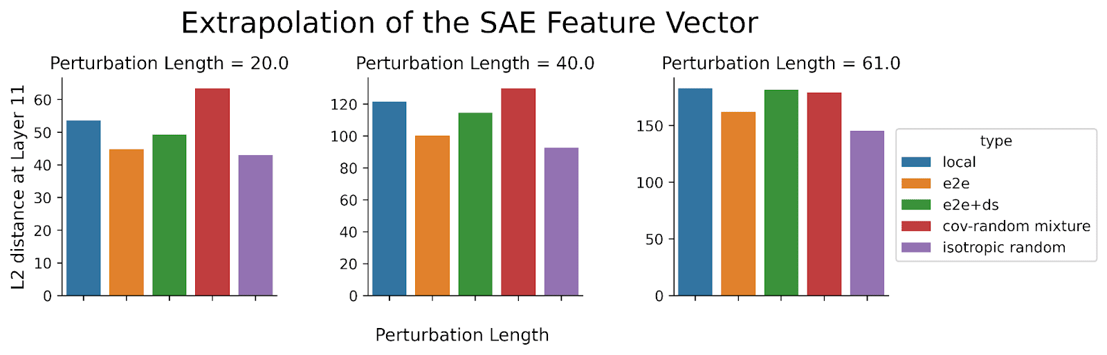
- We select a specific L0 value to conduct a more detailed comparison of the SAE models (L0 = 30.9 for local SAE, L0 = 27.5 for e2e SAE, and L0 = 31.4 for ds+e2e SAE). Among these, e2e SAE features have the least impact on the model output (Figure 8). At shorter perturbation lengths, local SAE features influence the model more than e2e+ds SAE features, but this difference shrinks as the perturbation lengths increase.
- Using the same L0 may not be a fair way to compare the three SAE models. This is because end-to-end SAEs are known to explain more network performance given the same L0 (Braun 2024).
- The result was initially surprising because we would have expected that end-to-end SAEs would more directly capture the features most crucial for token predictions. Our hypothesis for the explanation for this observation is that e2e SAE features perform worse because they are more isotropic (see Figure 3(a) from Braun 2024). Connecting this with the observation that perturbing along less meaningful directions leads to longer activation plateaus (Heimersheim 2024 [LW · GW]), it appears that e2e SAE minimizes the KL divergence between the original and reconstructed activations by exploiting the space outside the typical activation space. This could be an unintended and undesirable consequence of end-to-end SAEs—potentially the opposite of what we aim for in SAE features! While e2e SAE might exhibit this behavior, it is unclear to what extent e2e+ds SAE also does this.
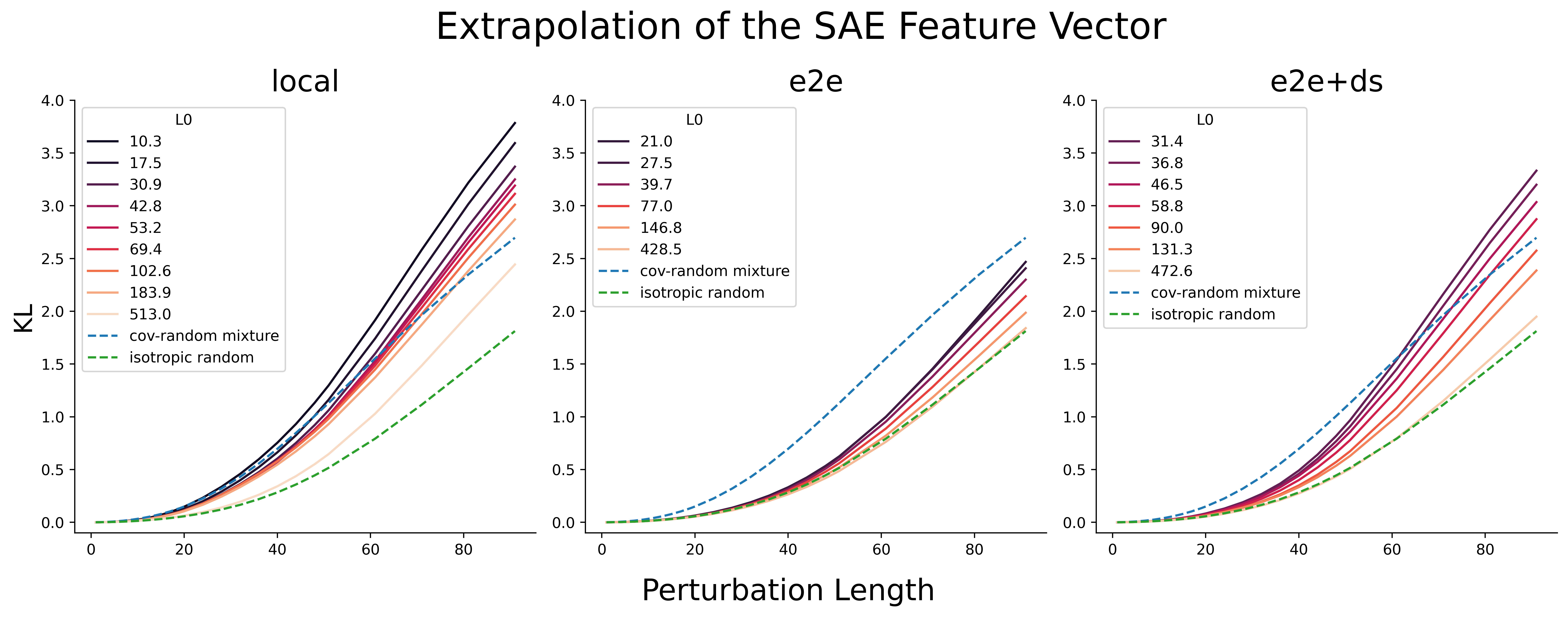
resid_pre. The x-axis is the perturbation length and the y-axis is the mean KL of logits. For the three columns, we compare the three different SAE model types. We compare the SAE feature directions with cov-random mixture and isotropic random directions. We color the lines by different L0 values of the SAEs.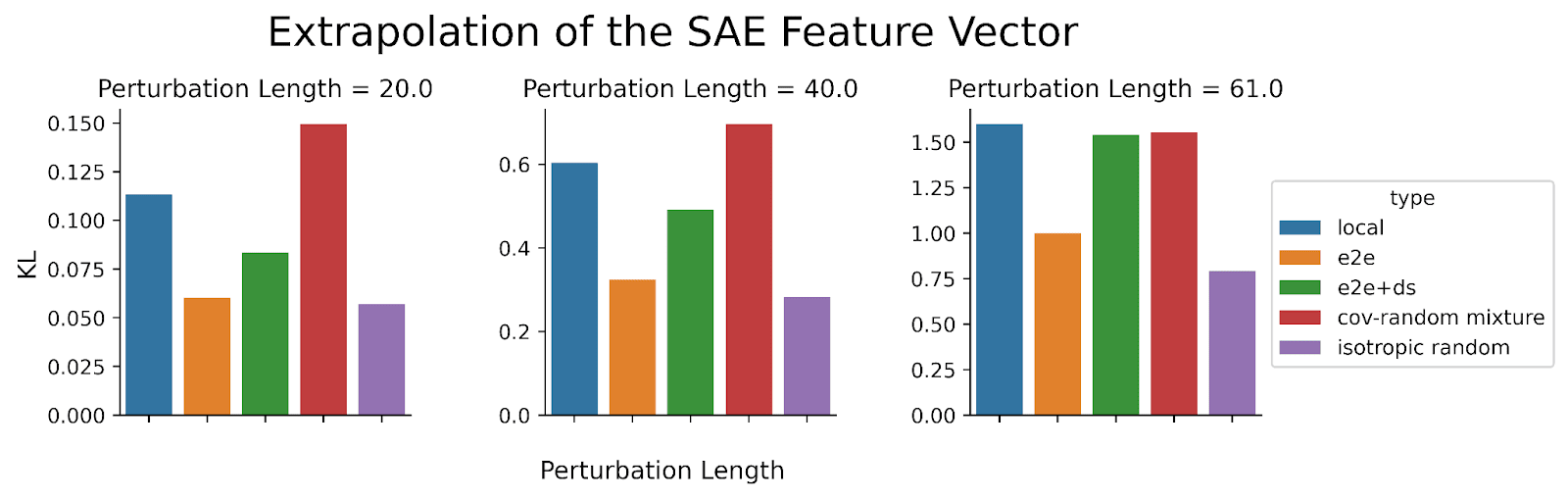
resid_pre. The x-axis is the direction type and the y-axis is the mean KL of logits. The features for local SAE generally induced the greatest change in the SAE models.Conclusion
Summary: We run sensitive direction experiments for various perturbations on GPT2-small activations. We find:
- SAE errors are no longer pathologically large when compared to more realistic baselines.
- Extrapolating SAE errors shows a different pattern for traditional SAEs versus end-to-end SAEs.
- Model is more sensitive to lower L0 SAE features.
- End-to-end SAE features do not exhibit stronger effect on the model output than traditional SAE features.
Limitations: In this post, we primarily use the mean (of KL or L2 distance) as our main measure. However, relying solely on the mean as a summary statistic might oversimplify the complexity of sensitive directions. For instance, the overall shape of the curve for each perturbation could be another important feature that we may be overlooking. While we did examine some individual curves and observed that real mixture and cov-random mixture generally exhibited greater model output change compared to isotropic random, the pattern was not as clear-cut.
Future Work:
- We are interested in further exploring why the average KL divergence for SAE(x) and cov-random mixture is not consistent across the different layers of GPT2-small. This may be a property of the cov-random mixture baseline, the SAE model, or the unique characteristic of some layers in GPT2-small.
- We want to explore what makes the model more sensitive to lower L0 SAE features. Understanding this might provide insights into how we can improve the training of SAEs.
- We want to consider whether we can develop a better "positive" baseline that represents a true feature direction. This could help refine our understanding and evaluation of SAE performance.
- We are considering whether using toy models could help us better understand how to leverage sensitive direction experiments for evaluating the true functional importance of features. This approach might provide clearer insights into the relationship between perturbations and feature relevance, potentially guiding us in refining our evaluation methods.
Acknowledgement: We thank Wes Gurnee for initial help with SAE error analysis and feedback on these results, Andy Arditi for useful feedback and discussion, Braun et al. and Joseph Bloom for SAEs used in this research, and Stefan Heimersheim’s LASR Labs team (Giorgi Giglemiani, Nora Petrova, Chatrik Singh Mangat, Jett Janiak) for helpful discussions.
Appendix
L2 Version of the Main Figures
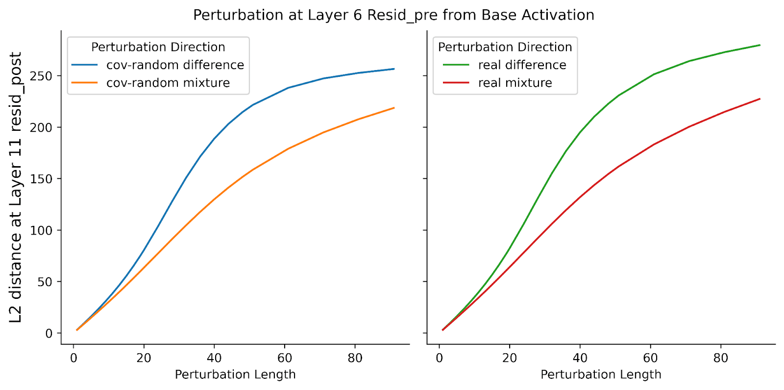
resid_pre. The x-axis is the perturbation length and the y-axis is the mean L2 distance at Layer 11 resid_post. For the plot in the left column, we compare “cov-random difference” and “cov-random mixture.” For the plot in the right column, we compare “real difference” and “real mixture.” For both cases, the “difference” perturbations have a greater change in model output than “mixture” perturbations.
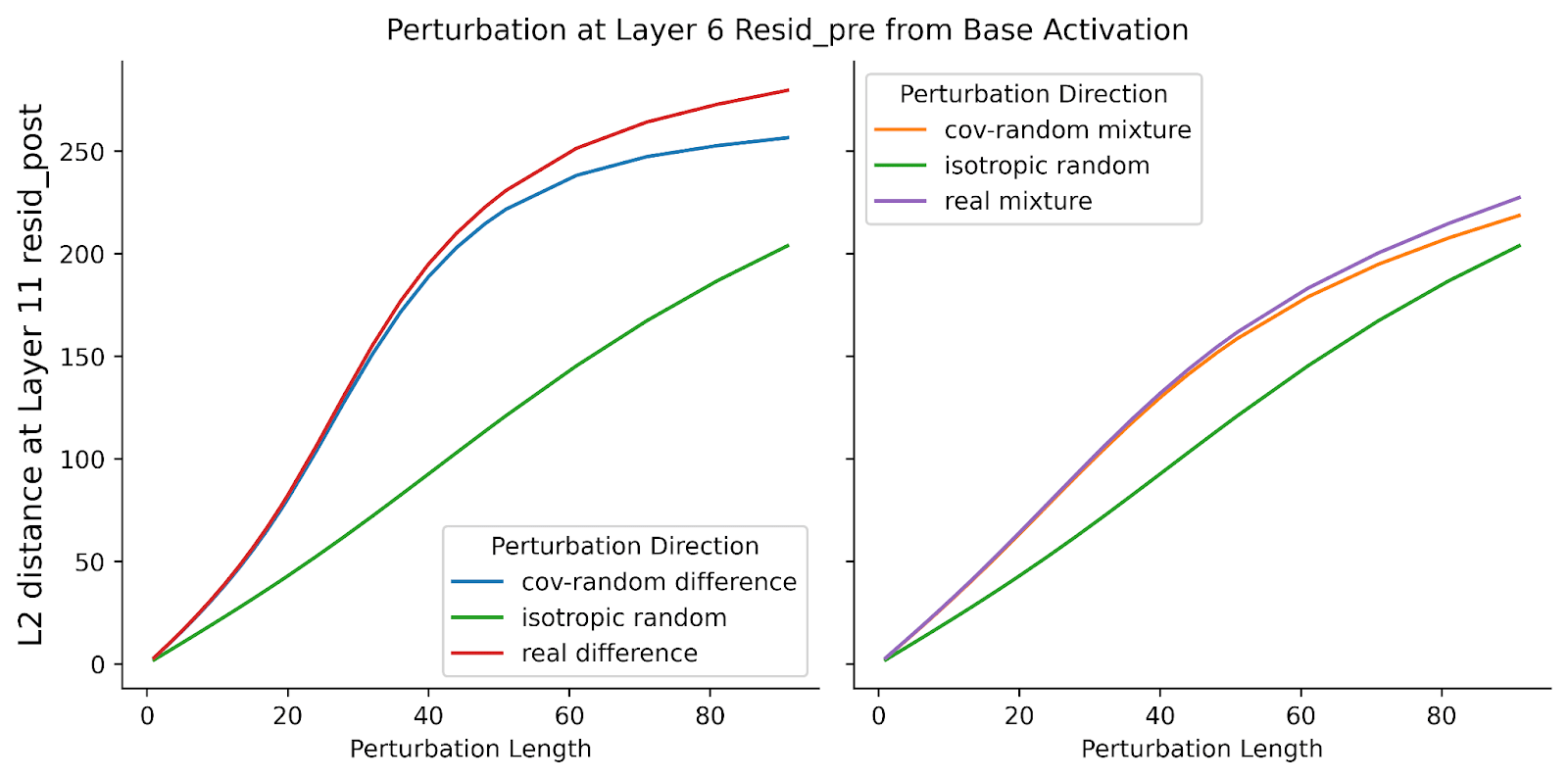
resid_pre. The x-axis is the perturbation length and the y-axis is the mean L2 distance at Layer 11 resid_post . On the right, we compare “isotropic difference,” “cov-random difference,” and “real mixture.” On the left, we compare “isotropic random,” “cov-random mixture,” and “real mixture.” “Cov-random mixture” induces a significantly greater change in model output than isotropic random. While the model is more sensitive to “real mixture” directions than the two other perturbation types, there is minimal difference between “real mixture” and “cov-random mixture.”
resid_pre. The x-axis is the perturbation length and the y-axis is the mean L2 distance at Layer 11 resid_post. For the three columns, we compare the three different SAE model types. We compare the SAE reconstruction error directions with cov-random mixture and isotropic random directions. We color the lines by different L0 values of the SAEs.
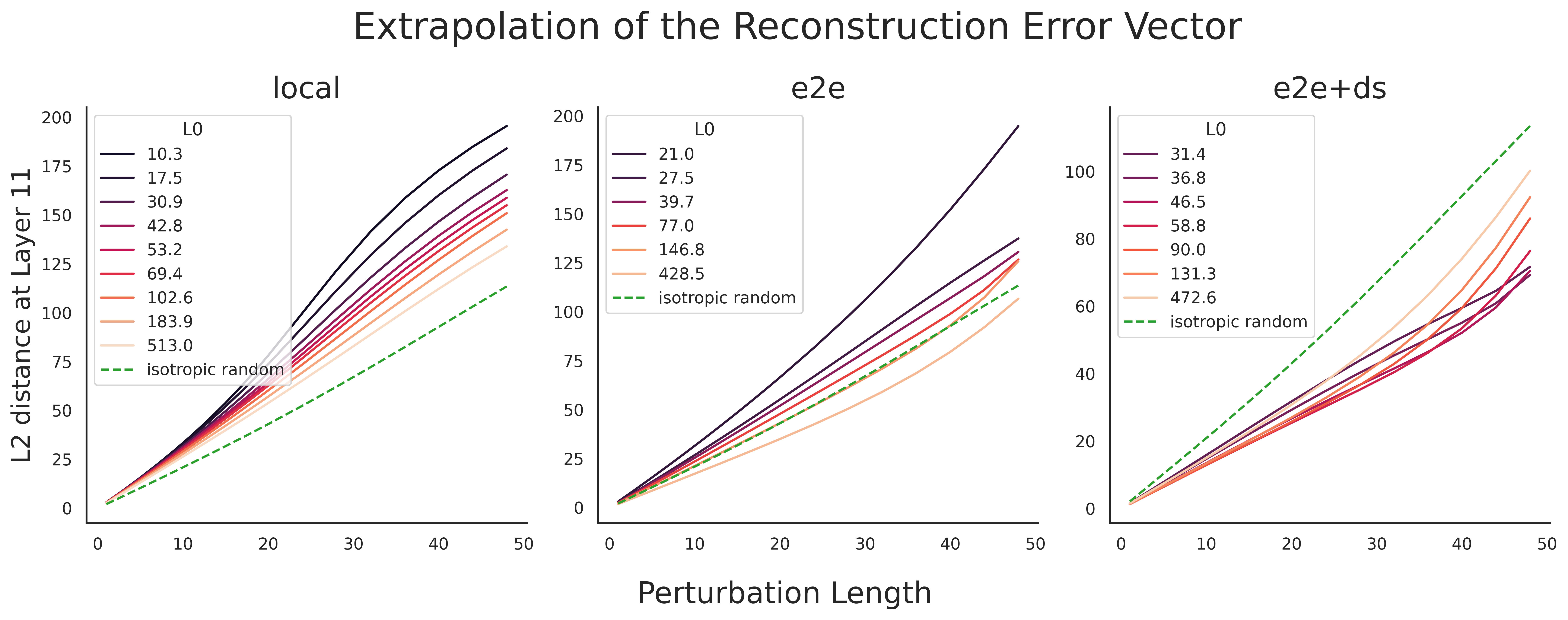
resid_pre. The x-axis is the perturbation length and the y-axis is the mean L2 distance at Layer 11 resid_post. For the three columns, we compare the three different SAE model types. We compare the SAE reconstruction error directions with isotropic random directions. We color the lines by different L0 values of the SAEs. Note that the y-axis limit is not the same for the three plots.
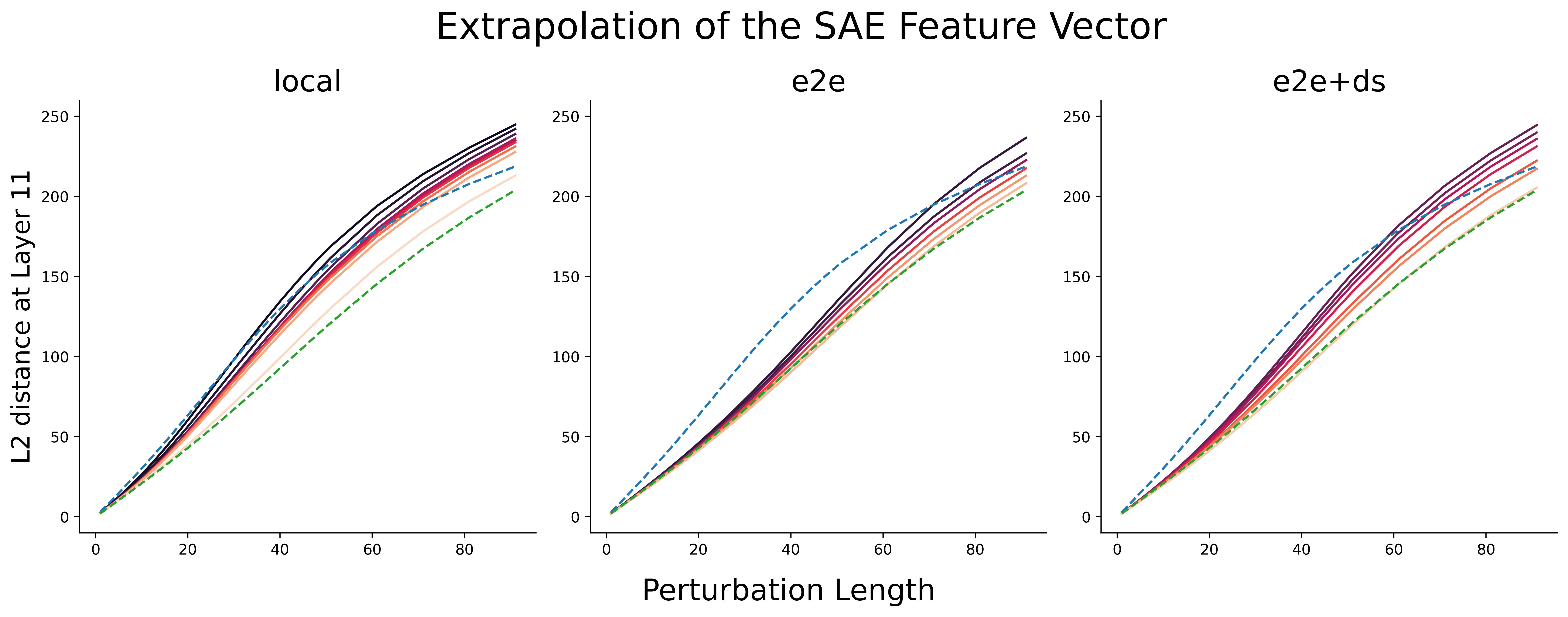
resid_pre. The x-axis is the perturbation length and the y-axis is the mean L2 distance at Layer 11 resid_post. For the three columns, we compare the three different SAE model types. We compare the SAE feature directions with cov-random mixture and isotropic random directions. We color the lines by different L0 values of the SAEs.
resid_pre. The x-axis is the direction type and the y-axis is the mean L2 distance at Layer 11 resid_post. Local SAEs generally exhibited the greatest change for the SAE models.
Supplementary Figures
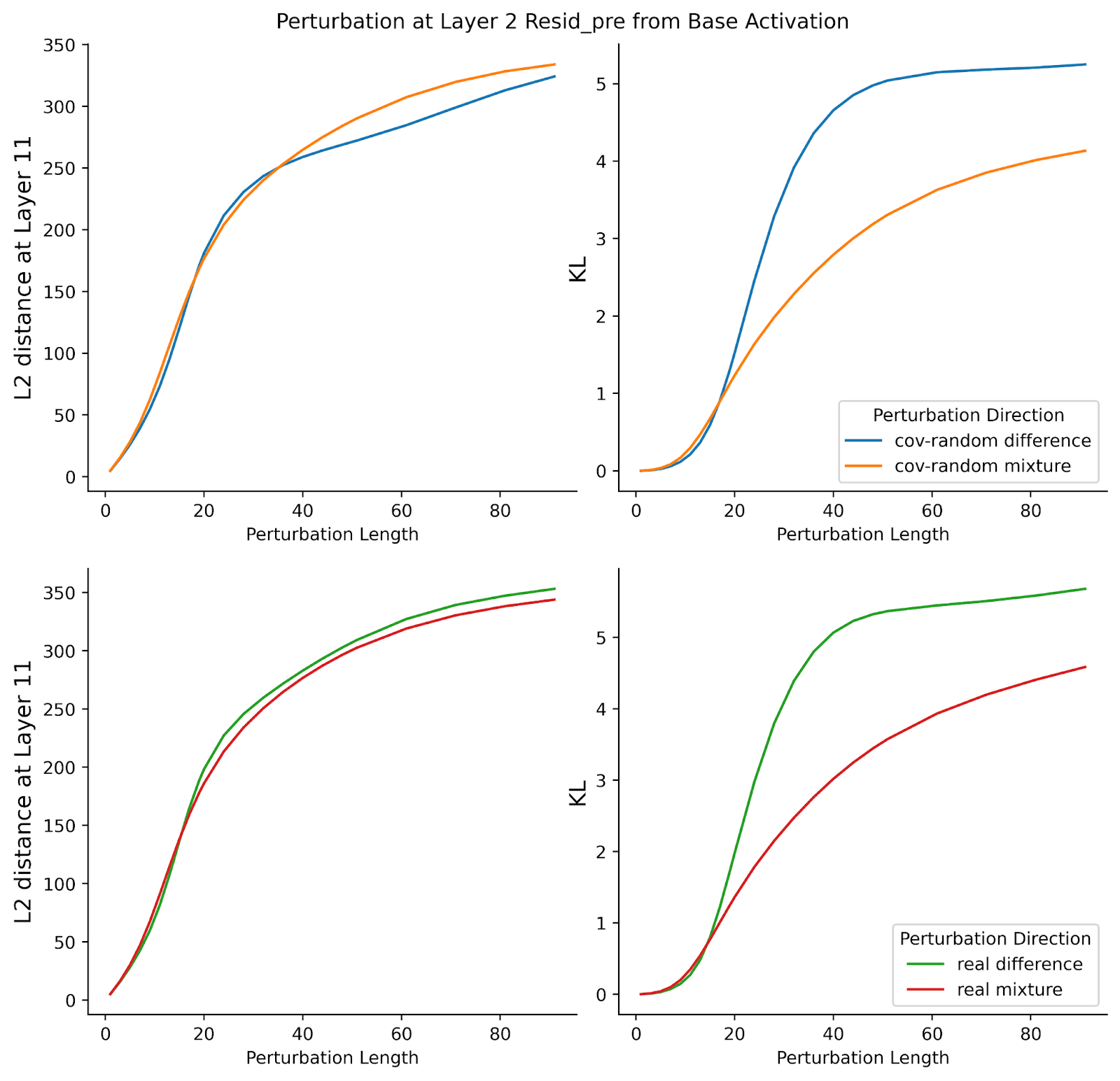
resid_pre. The x-axis is the perturbation length and the y-axis is the mean L2 distance at Layer 11 resid_post (left column) or mean KL of logits (right column). For the plots in the top row, we compare “cov-random difference” and “cov-random mixture.” For the plots in the bottom row, we compare “real difference” and “real mixture.” For both cases, the “difference” perturbations have a greater change in model output than “mixture” perturbations. However, the differences in L2 distance at Layer 11 is much smaller than the perturbations in Layer 6.
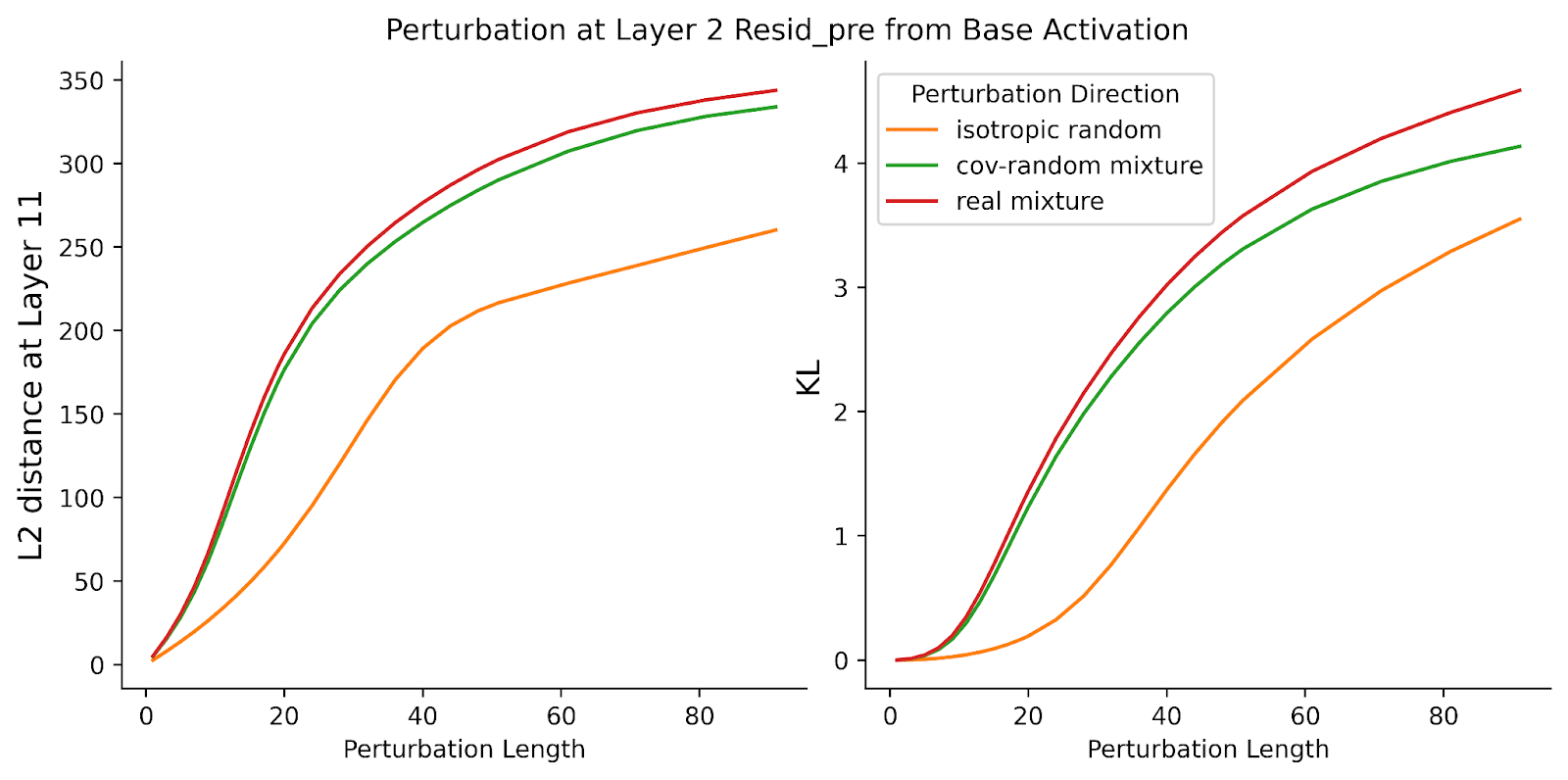
resid_pre. The x-axis is the perturbation length and the y-axis is the mean L2 distance at Layer 11 resid_post (left column) or mean KL of logits (right column). We compare “isotropic random,” “cov-random mixture,” and “real mixture.” “Cov-random mixture” induces a significantly greater change in model output than isotropic random. While the model is more sensitive to “real mixture” directions than the two other perturbation types, there is minimal difference between “real mixture” and “cov-random mixture,” especially for the L2 distance.
- ^
In general we observed that perturbations including the negative of the original activation have stronger, qualitatively different, effects.
0 comments
Comments sorted by top scores.