Characterizing stable regions in the residual stream of LLMs
post by Jett Janiak (jett), jacek (jacek-karwowski), Chatrik (csmyo22), Giorgi Giglemiani (Rakh), nlpet, StefanHex (Stefan42) · 2024-09-26T13:44:58.792Z · LW · GW · 4 commentsThis is a link post for https://arxiv.org/abs/2409.17113
Contents
4 comments
This research was completed for London AI Safety Research (LASR) Labs 2024. The team was supervised by @Stefan Heimershiem [LW · GW] (Apollo Research). Find out more about the program and express interest in upcoming iterations here.
This video is a short overview of the project presented on the final day of the LASR Labs. Note that the paper was updated since then.
We study the effects of perturbing Transformer activations, building upon recent work by Gurnee [AF · GW], Lindsey, and Heimersheim & Mendel [LW · GW]. Specifically, we interpolate between model-generated residual stream activations, and measure the change in the model output. Our initial results suggest that:
- The residual stream of a trained Transformer can be divided into stable regions. Within these regions, small changes in model activations lead to minimal changes in output. However, at region boundaries, small changes can lead to significant output differences.
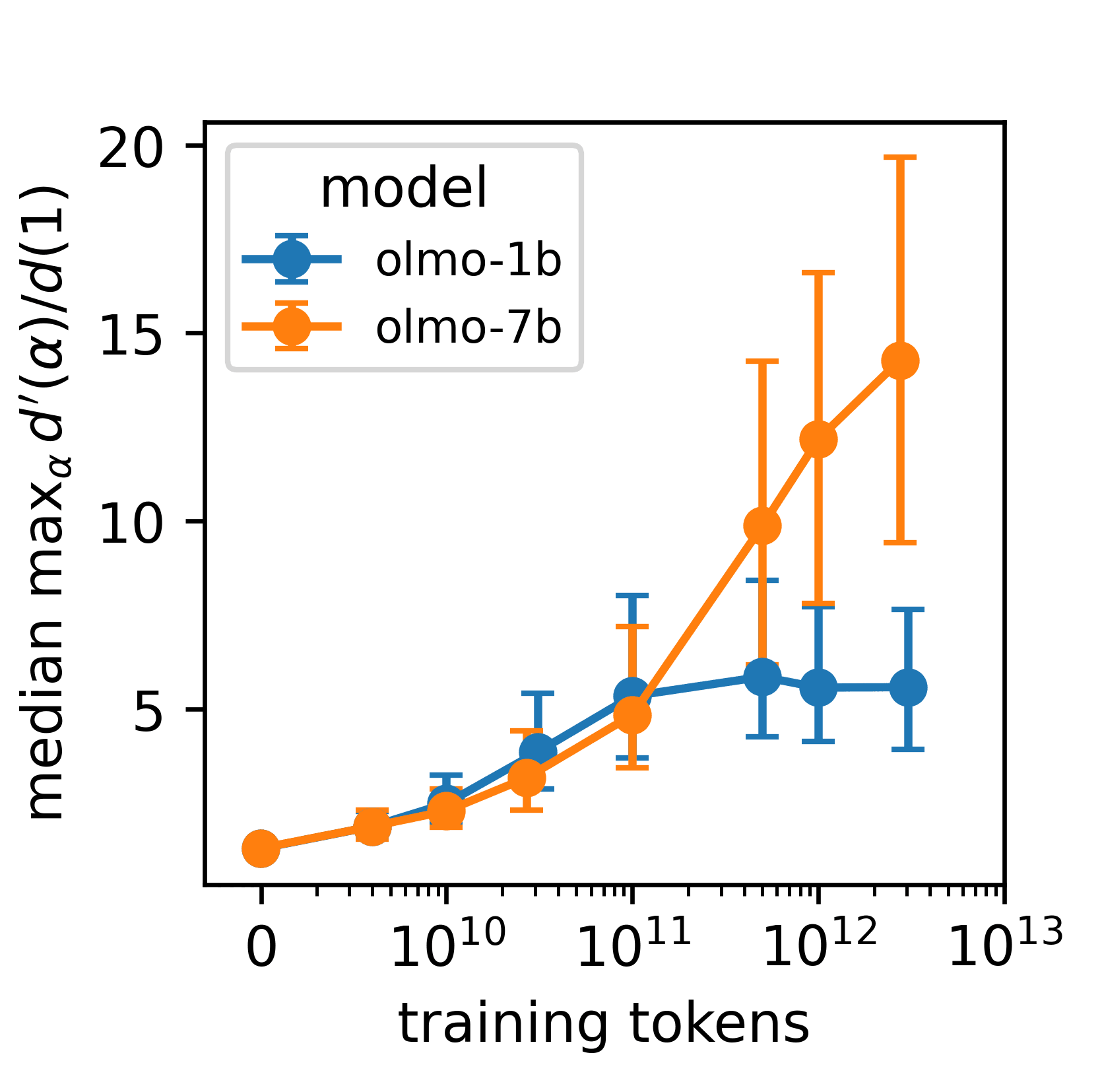
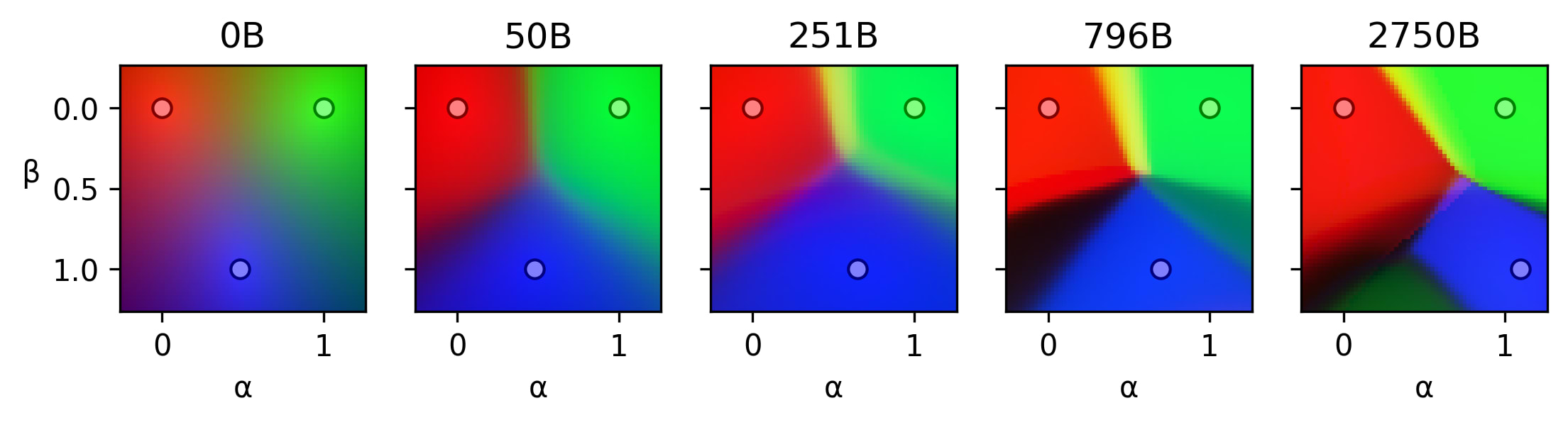
- These regions emerge during training and evolves with model scale. Randomly initialized models do not exhibit these stable regions, but as training progresses or model size increases, the boundaries between regions become sharper.
- These stable regions appear to correspond to semantic distinctions. Dissimilar prompts occupy different regions, and activations from different regions produce different next token predictions.
- While further investigation is needed, these regions appear to be much larger than polytopes studied by Hanin & Rolnick and Black et al. [LW · GW]
We believe that studying stable regions can improve our understanding of how neural networks work. The extent to which this understanding is useful for safety is an active topic of discussion 1 [LW · GW] 2 [LW · GW] 3 [LW · GW].
You can read the paper on arxiv.
4 comments
Comments sorted by top scores.
comment by gwern · 2024-09-26T16:20:12.965Z · LW(p) · GW(p)
Is this consistent with the interpretation of self-attention as approximating (large) steps in a Hopfield network?
Replies from: jett↑ comment by Jett Janiak (jett) · 2024-09-27T12:26:04.740Z · LW(p) · GW(p)
I'm not familiar with this interpretation. Here's what Claude has to say (correct about stable regions, maybe hallucinating about Hopfield networks)
This is an interesting question that connects the findings in the paper to broader theories about how transformer models operate. Let me break down my thoughts:
The paper's findings and the Hopfield network interpretation of self-attention are not directly contradictory, but they're not perfectly aligned either. Let's examine this in more detail:
- The paper's key findings:
- The residual stream of trained transformers contains stable regions where small activation changes lead to minimal output changes.
- These regions emerge during training and become more defined as training progresses or model size increases.
- The regions appear to correspond to semantic distinctions.
- The Hopfield network interpretation of self-attention:
- Self-attention layers in transformers can be seen as performing energy-based updates similar to those in continuous Hopfield networks.
- This view suggests that self-attention is performing pattern completion or error correction, moving activations towards learned attractor states.
Now, let's consider how these might relate:
- Consistency with stable regions: The existence of stable regions in the residual stream could be consistent with the idea of attractor states in a Hopfield-like network. The stable regions might correspond to basins of attraction around these states.
- Emergence during training: The paper observes that stable regions emerge and become more defined during training. This aligns well with the Hopfield network interpretation, as training would refine the attractor landscapes.
- Semantic correspondence: The paper suggests that stable regions correspond to semantic distinctions. This is compatible with the Hopfield network view, where different attractor states could represent different semantic concepts or categories.
- Sharp transitions: The paper observes sharp transitions between stable regions. This is somewhat less aligned with the typical continuous Hopfield network dynamics, which often show smoother transitions. However, it's not necessarily inconsistent, as the observed behavior could result from complex interactions across multiple layers.
- Scale of regions: The paper suggests that these stable regions are much larger than previously studied polytopes. This might pose some challenges for the Hopfield network interpretation, as it implies a different granularity of representation than might be expected.
comment by Jett Janiak (jett) · 2024-09-26T13:49:52.388Z · LW(p) · GW(p)
I believe there are two phenomena happening during training
- Predictions corresponding to the same stable region become more similar, i.e. stable regions become more stable. We can observe this in the animations.
- Existing regions split, resulting in more regions.
I hypothesize that
- could be some kind of error correction. Models learn to rectify errors coming from superposition interference or another kind of noise.
- could be interpreted as more capable models picking up on subtler differences between the prompts and adjusting their predictions.
comment by J Bostock (Jemist) · 2024-09-26T14:54:26.071Z · LW(p) · GW(p)
I have an old hypothesis about this which I might finally get to see tested. The idea is that the feedforward networks of a transformer create little attractor basins. Reasoning is twofold: the QK-circuit only passes very limited information to the OV circuit as to what information is present in other streams, which introduces noise into the residual stream during attention layers. Seeing this, I guess that another reason might be due to inferring concepts from limited information:
Consider that the prompts "The German physicist with the wacky hair is called" and "General relativity was first laid out by" will both lead to "Albert Einstein". Both of them will likely land in different parts of an attractor basin which will converge.
You can measure which parts of the network are doing the compression using differential optimization, in which we take d[OUTPUT]/d[INPUT] as normal, and compare to d[OUTPUT]/d[INPUT] when the activations of part of the network are "frozen". Moving from one region to another you'd see a positive value while in one basin, a large negative value at the border, and then another positive value in the next region.