Residual stream norms grow exponentially over the forward pass
post by StefanHex (Stefan42), TurnTrout · 2023-05-07T00:46:02.658Z · LW · GW · 24 commentsContents
  Plots showing exponential norm and variance growth
  Comparison of various transformer models
    BOS and padding tokens
  Theories for the source of the growth
  Analyzing the model weights to understand the behaviour
    Analyzing the Attention weights
    Analyzing the MLP weights
  Why an exponential residual stream norm increase might be useful
  Conclusion
      Contributions:
    Appendix 1: Attention+MLP contribution norms must exceed block-over-block norm growth rate
    Appendix 2: Explaining the difference between attn_out and mlp_out
    Appendix 3: Which of the MLP weights are the source of the exponential growth?
None
24 comments
Summary: For a range of language models and a range of input prompts, the norm of each residual stream grows exponentially over the forward pass, with average per-layer growth rate of about 1.045 in GPT2-XL. We show a bunch of evidence for this. We discuss to what extent different weights and parts of the network are responsible.
We find that some model weights increase exponentially as a function of layer number. We finally note our current favored explanation: Due to LayerNorm, it's hard to cancel out existing residual stream features, but easy to overshadow existing features by just making new features 4.5% larger.
Thanks to Aryan Bhatt, Marius Hobbhahn, Neel Nanda, and Nicky Pochinkov for discussion.
Plots showing exponential norm and variance growth
Our results are reproducible in this Colab.
Alex noticed exponential growth in the contents of GPT-2-XL's residual streams. He ran dozens of prompts through the model, plotted for each layer the distribution of residual stream norms in a histogram, and found exponential growth in the norm of the residual streams:
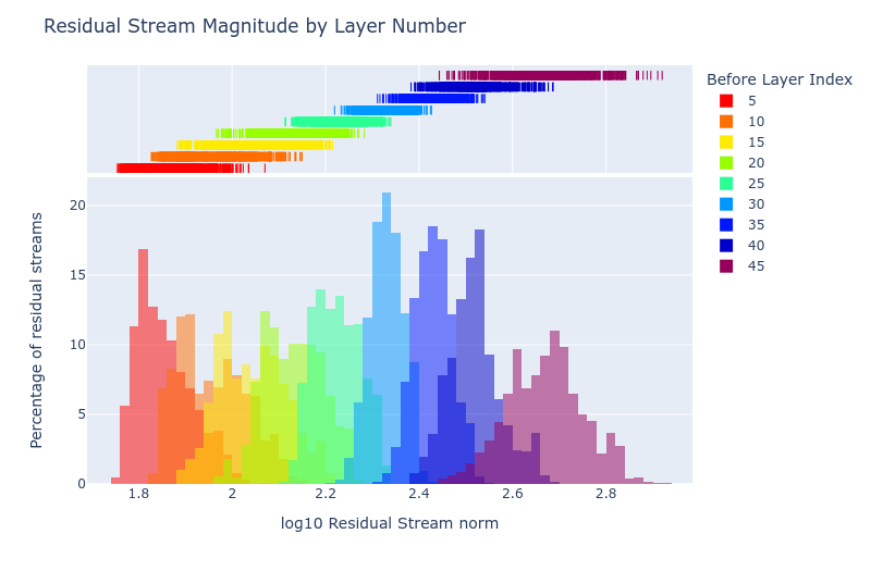
GPT2-XL has 48 layers in total.
Here's the norm of each residual stream for a specific prompt:
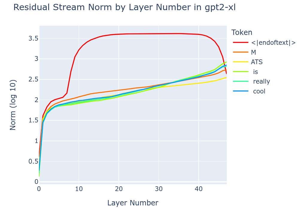
<|endoftext|>) behaves differently, which is why we exclude it from the averaged plots.Stefan had previously noticed this phenomenon in GPT2-small, back in MATS 3.0:
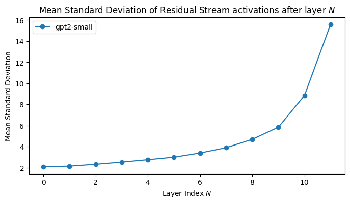
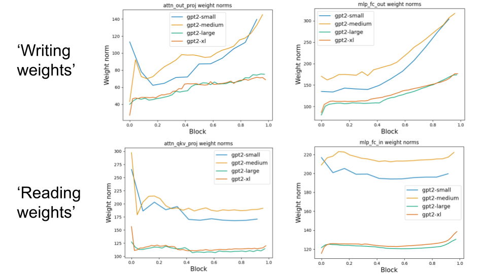
Basic Facts about Language Model Internals [LW · GW] also finds a growth in the norms of the attention-out matrices and the norms of MLP out matrices ("writing weights"), while they find stable norms for , , and ("reading weights"):
Comparison of various transformer models
We started our investigation by computing these residual stream norms for a variety of models, recovering Stefan's results (rescaled by ) and Alex's earlier numbers. We see a number of straight lines in these logarithmic plots, which shows phases of exponential growth.
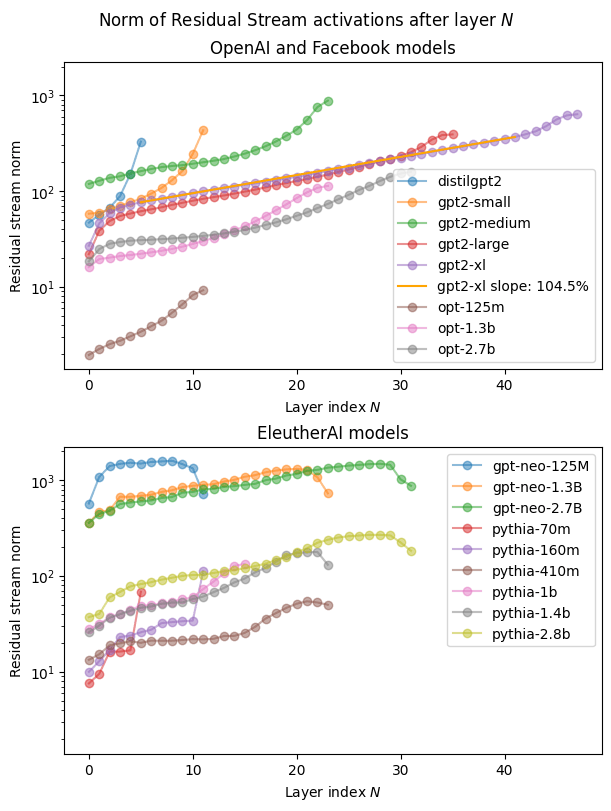
We are surprised by the decrease in Residual Stream norm in some of the EleutherAI models.[2] We would have expected that, because the transformer blocks can only access the normalized activations, it's hard for the model to "cancel out" a direction in the residual stream. Therefore, the norm always grows. However, this isn't what we see above. One explanation is that the model is able to memorize or predict the LayerNorm scale. If the model does this well enough it can (partially) delete activations and reduce the norm by writing vectors that cancel out previous activations.
The very small models (distillgpt2, gpt2-small) have superexponential norm growth, but most models show exponential growth throughout extended periods. For example, from layer 5 to 41 in GPT2-XL, we see an exponential increase in residual stream norm at a rate of ~1.045 per layer. We showed this trend as an orange line in the above plot, and below we demonstrate the growth for a specific example:
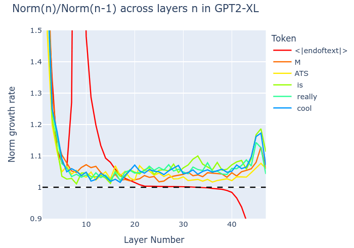
<|endoftext|> (BOS) token at residual stream position 0. Its growth rate (shown in red) is huge at first, but represents an exception as noted before. The dashed line indicates a growth rate of 1 (constant norm). Since the (non-
<|endoftext|>) growth rates are approximately constant and above the line, the residual streams are growing exponentially.BOS and padding tokens
In our initial tests, we noticed some residual streams showed a irregular and surprising growth curve:
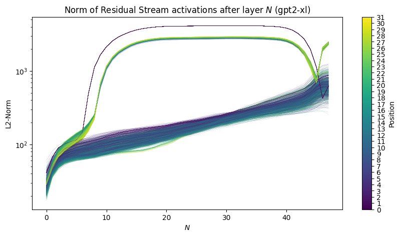
As for the reason behind this shape, we expect that the residual stream (norm) is very predictable at BOS and padding positions. This is because these positions cannot attend to other positions and thus always have the same values (up to positional embedding). Thus it would be no problem for the model to cancel out activations, and our arguments about this being hard do not hold for BOS and padding positions. We don't know whether there is a particular meaning behind this shape.
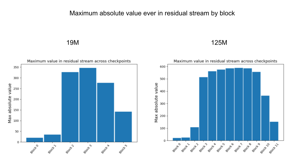
We suspect that is the source of the U-shape shown in Basic facts about language models during training [LW · GW]:
Theories for the source of the growth
From now on we focus on the GPT2-XL case. Here is the residual stream growth curve again (orange dots), but also including the resid_mid hook between the two Attention and MLP sub-layers (blue dots).
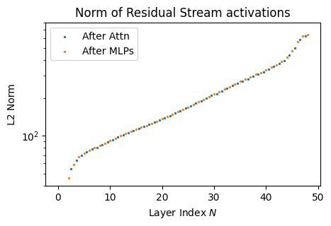
Our first idea upon hearing exponential growth was:
Each OV circuit is a linear function of the residual stream given a fixed attention pattern. Then you add the head OV outputs back into a residual stream, which naively doubles the magnitude assuming the OV outputs have similar norm to the input residual stream. That produces exponential growth.
However, we think that this does not work due to LayerNorm (LN). With LayerNorm, the input into the Attention and MLP sub-layers is normalized to have standard deviation 1 and norm (neglecting the learned LN parameters, which we discuss in footnote [3]). Despite this, the Attention and MLP sub-layers have output contributions which increase proportionally to the overall residual stream norm that is exponentially increasing.
We can think of two ways to get exponential growth of the residual stream despite LN:
- The Attention and/or MLP weights and/or LN parameters can just be higher in later layers (following this exponential rate). This is something the model could learn in training, essentially making sure the Attention and MLP outputs grow by 4.5% per layer, independently of the residual stream norm.
- Sneaking information through the LayerNorm. Maybe there is a hidden property (say "number of features") that is not affected by LN but that causes the typical exponential growth "Attention/MLP output proportional is to the number of features". Note that this theory requires (i) LN does not reduce the number of features, but (ii) the number of features affects the norm of Attention/MLP output.
To illustrate the second theory, consider the following toy example where and have the same norm, but contains only one feature (the "alternating" feature) while contains two features (the "alternating" feature, and the "1st != 3rd number" feature).
This way, a property (number of features) can be hidden in the inputs (hidden as in, the inputs have identical norms), and affect the norms of the outputs. This works less nicely with ReLU or GELU but the output norms still differ.
To distinguish these two theories, we can test whether we see an exponential increase in the norm of Attention/MLP weights, or alternatively, an exponential increase in the norm of Attention/MLP outputs on random layer-independent inputs. Either of these would mean we don't need theory 2's sneaking features-shenanigans and can explain the exponential growth as being "hard-coded" into the model weights.
Note: It's possible for just one of the sub-layer types (Attention or MLP) to grow exponentially and still cause the overall exponential growth (see appendix 1 [LW · GW] for a related proof). But this seems unlikely as the non-exponential sub-layer would lose impact on the residual stream, and we expect the model to make use of both of them. Indeed, plotting the outputs attn_out and mlp_out shows both increasing at the exponential rate (but attn_out seems to fall off at layer ~30).
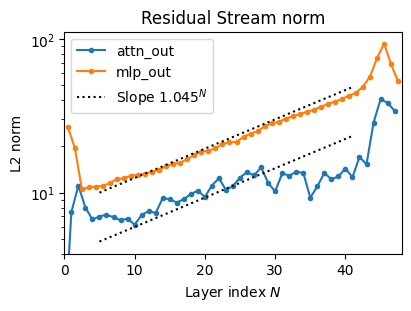
attn_out and mlp_out, see appendix 2 [LW · GW].Analyzing the model weights to understand the behaviour
We want to know why the residual stream norm is growing. Is it some process that naturally creates an exponential increase (maybe features accumulating in the residual stream)—and how would that work? Or are the weights[3] of later layers inherently larger and thus cause larger outputs?
We know that both attn_out and mlp_out grow exponentially. In the next two section we look at the Attention and MLP weights, respectively.
TL;DR: We do find evidence for exponentially increasing weights in both sub-layers, although in both cases we are somewhat confused what is happening.
Analyzing the Attention weights
What do want to get evidence on? We want to know why attn_out grows exponentially with layer number: Is the growth a property inherent to the Attention weights in each of the layers (theory 1), or is the growth relying on properties of the residual stream (theory 2).
What test do we run and why does that give us evidence? We test whether the Attention OV-circuit weights grow exponentially with layer number, at the same rate as the actual Attention outputs attn_out. If true, this is evidence for theory 1.
The Attention layer output attn_out is determined by the QK-circuits (select which inputs to attend to), and the OV-circuits (determine how the inputs are transformed). For the purposes of understanding the overall residual stream growth—why the outputs have larger norm than the inputs—we want to focus on the OV-circuits, which determine how the norm changes from input to output.
The OV-circuits consist of the matrices (product of the value and output matrices) and the bias .[4] There are 25 attention heads in GPT2-XL, i.e. 25 matrices. In the figure below we plot the Frobenius norm[5] of the matrices (grey solid lines) and L2 norm of the vector (pink line), and compare it to the L2 norm of attn_out (blue solid line).
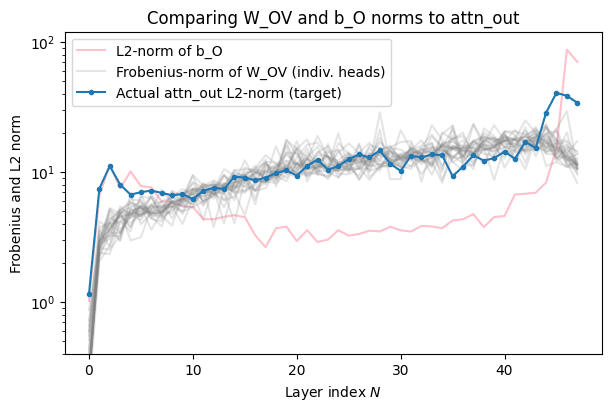
attn_out? We see the norms increase at the same rate as the attn_out normsThe Frobenius norms of the attention heads (grey lines) match the actual attn_out norms (blue line) somewhat accurately, and grow exponentially. The bias term (pink line) seems mostly negligible except for in the final layers.
What did we find? We find that the Attention weights, specifically the norms, grow approximately exponentially at the rate of attn_out. This is evidence for theory 1 because it means that the model bothered to learn weights that increase exponentially with layer number. [6]
Caveats: We do not understand the full picture of how attn_out is generated, all we notice is that they grow at the same rate.
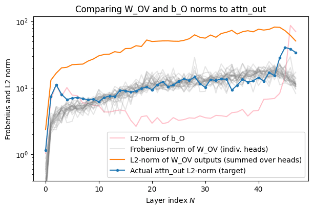
What we would have liked: We show that any normalized random input into Attention layer N leads to an Attention output of the observed norm.
What we got: For some unit-normalized, Gaussian-sampled vector , consider the sum of the sum of for all 25 matrices (one for each head). This sum's norm is 5 times larger than the attn_out norm, as shown in the figure. [7]
Analyzing the MLP weights
What do want to get evidence on? We want to know why mlp_out grows exponentially with layer number: Is the growth a property inherent to the MLP weights in each of the layers (theory 1), or is the growth relying on properties of the residual stream (theory 2).
What test do we run and why does that give us evidence? We test whether feeding layer-independent inputs to the MLPs produces outputs that do scale exponentially with layer, in a way which follows the exponential growth of mlp_out.
If this is true, this is evidence for theory 1 and against theory 2. If this is false, we cannot draw strong evidence from this.
We do not attempt to find the right way to combine model weights into a "norm" of the MLP layer. Instead, we draw input vectors from a Normal distribution, and normalize them to mean 0 and variance 1. We feed these vectors into the MLP. [8]
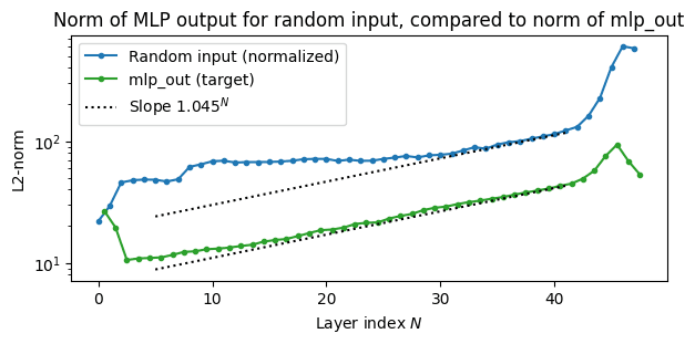
What did we find? We find that the MLP outputs of normalized random Gaussian inputs do scale exponentially with layer numbers, for layers 30 - 43, at the same rate as mlp_out. This is evidence for theory 1.
Caveats: We do not reproduce the mlp_out norms but find a much larger output norm with the random inputs. We discuss this further in an appendix, but the bottom line is that random vectors are indeed qualitatively different from residual stream vectors, and notably random vectors cause 4x more of the GELU activation to be active (>0) than normal residual stream vectors. (On the second theory—do random vectors have "more features", and thus higher norm?)
Why an exponential residual stream norm increase might be useful
Transformers might sometimes want to delete information from the residual stream, maybe to make space for new information. However, since all blocks only receive the normalized (LayerNorm) residual stream, it may be impossible to do deletions the intuitive way of "just write to the residual stream" to delete a vector . It might approximately work if the model can predict the LayerNorm scale, but it seems hard to do accurately.
Alternatively, the model could write all new information with an increased norm. An exponential growth would make the most recent layers have an exponentially larger effect on the residual stream at any given layer.
However, this is complicated by weight decay, which is a term in the loss that penalizes large weight magnitudes. While we analyzed GPT2-XL's weights in this post, we also earlier displayed similar residual stream norm trends for a range of models. The OPT and GPT-Neo models were trained with weight decay of 0.1, while the Pythia models were trained with 0.01. We don't know about distilgpt2 or the normal GPT2-series. If models trained with weight decay still exhibit weight norms which increase exponentially with layer number, then that means something is happening which somehow merits an exponential hit to loss.[9]
ETA 5/7/23: Apparently, LN parameters are often excluded from weight decay. (For example, see the minGPT implementation.) This means that the gain parameters can freely magnify the LN output, without incurring extra regularization loss. (However, this also suggests that W_in and W_OV should in general become extremely tiny, up to precision limits. This is because their norm can be folded into the LN parameters in order to avoid regularization penalties.)
Conclusion
We documented a basic tendency of transformers: residual stream variance grows exponentially. We think that a big chunk of the exponential increase does come from the model weights, but have not fully understood the underlying mechanics (e.g. GELU activation rates).
Contributions:
Stefan (StefanHex) wrote a lot of the post, noticed this in GPT2-small, compared the phenomenon between models, and did the analysis of activations and weights.
Alex (TurnTrout) wrote some of the post and edited it, noticed the phenomenon in GPT2-XL, made about half of the assets and some of the hooking code for computing residual stream norms. He also wrote appendix 1.
Appendix 1: Attention+MLP contribution norms must exceed block-over-block norm growth rate
Proposition: Attention + MLP norm contributions must exceed the growth rate.
Consider residual streams for the activation vector just before transformer layer , in a transformer where the MLP comes after the Attention sublayer. Suppose that, for layer , for growth rate . Then
Proof.
Then
QED.
For example, if , then the norms of the attention and MLP contributions must together be at least 5% of the norm of the resid_pre for layer .
Appendix 2: Explaining the difference between attn_out and mlp_out
Remembering the two plots from Theories for the source of the growth, we notice a surprisingly large y-axis difference between the norms. We repeat those norm curves here:
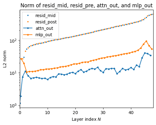
Now we show the same lines again, but switch to using the standard deviation. This is equivalent[1] (norm divided by standard deviation = ) but more intuitive to reason about. We also divide all lines by to make the lines fit better into the plot. The difference from resid_pre to resid_post at each layer has to be approximately a factor for 1.045 for the exponential growth to hold.
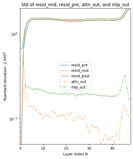
Intuitively, we expected these standard deviations to add up like those of independent (Gaussian) random vectors, ("error propagation" formula), but this doesn't work. We realized that correlated random vectors can have a higher summed variance, up to a maximum of . It would be interesting to see where in that range attn_out and mlp_out lie, i.e. how correlated the Attention and MLP outputs are with the residual stream input.
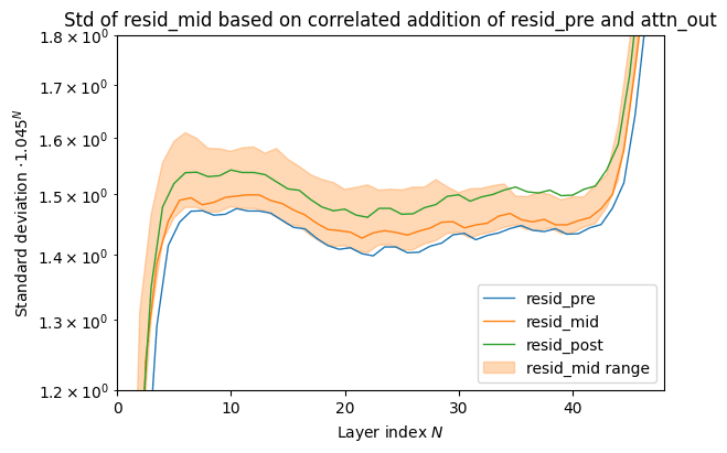
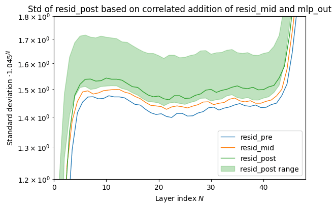
In both plots we see that the uncorrelated addition of residual stream and sub-layer output (lower end of the range) is much lower that required, providing nowhere near the observed growth for the residual stream. Our (somewhat extreme) upper end of the range is much larger, so if attn_out or mlp_out were perfectly proportional to their input residual stream we would see a much larger growth.
This does not directly affect our argument, which relies on just realizing the exponential growth at various points. We shared this since we initially did not take into account the correlation, and found this interesting.
Appendix 3: Which of the MLP weights are the source of the exponential growth?
We showed that the MLP output for random layer-independent inputs grows exponentially with layer number. This proves that there is something inherent to the MLP weights in each layer that causes the output to grow, but it does not show us what that is. The behaviour should be predictable from the MLP weights , , , and . In this section we want to show our investigation into this question, even though we have not completely solved it. This will also explain the large difference in norm between the random-input MLP output, and the actual-model MLP output we showed (figure from above inserted again)
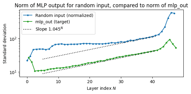
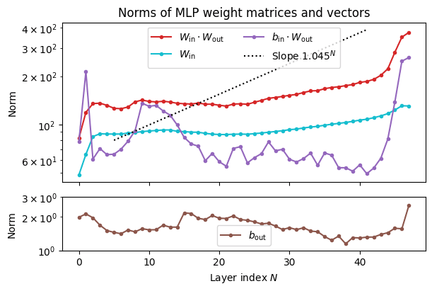
Our first step is to plot the norms of the individual MLP weight components. We are very surprised to not see any exponential increase at the expected rate in any of these norms!
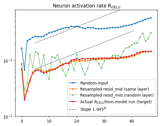
The other important part of an MLP layer is the non-linear activation function, in our case GELU. It turns out that the average neuron activation rate, i.e. the fraction of hidden neurons with pre-activation values >0 rises exponentially throughout the network! This is an essential component to the exponential growth of resid_out, and we did not notice this trend in any of the weight matrix norms. Note however that we only observe this exponential growth here from layer 5 til ~20.
In the plot below we see that even the neuron activation rate for random inputs (blue line) rises exponentially, so the exponential increase is still inherent to the layer weights, it was just not visible in the norms.
The plot below also explains the difference in L2 norm between actual mlp_out and the random outputs (the first plot in this appendix): The neuron activation rate is simply much higher for random inputs (blue line) than in the actual model run (red line), or for randomly-resampled[10] residual stream inputs (orange and green lines). The random vectors clearly differ from actual residual stream vectors in some significant way, but we have not investigated this further.
- ^
Note on norm, variance, and mean of the residual stream: All our models' residual streams have mean zero. One can always rewrite the model weights to make the residual stream mean zero, by subtracting the mean of weights from the weights themselves. We use the TransformerLens library which does this by default (
center_writing_weights). Then the L2 norm and variance or standard deviation are relatedwith the residual stream size .
- ^
According to the model card, the Pythia models have "exactly the same" architectures as their OPT counterparts.
- ^
Note that we fold together the LayerNorm weights with the following or weights. So when we show an exponential increase in, say, weights this might actually be fully or partially coming from the LayerNorm weights. It does not make a conceptual difference (the model still stores exponentially increasing weights), but may affect regularization.
That is, after each residual stream is set to mean 0 and std 1, LN applies learned gain parameters. If the residual stream norm can be recovered using these gain parameters, then there are only such parameters to scale (and thus penalize). But if has to amplify the post-LN residual stream, then there are parameters which would have to be scaled up by the same amount. This roughly seems like a quadratic increase in the regularization term in the loss function, but this is just a heuristic guess.
ETA 5/7/23: Apparently LN parameters are not, in general, weight-decayed.
- ^
Note that the value-bias is set to zero in TransformerLens, using another weight-rewrite trick.
- ^
According to Stefan's experimental data, the Frobenius norm of a matrix is equivalent to the expectation value of the L2 vector norm of for a random vector (sampled from normal distribution and normalized to mean 0 and variance 1). So calculating the Frobenius norm seems equivalent to testing the behaviour on random inputs. Maybe this is a theorem?
- ^
If GPT-2 is using weight decay, then the model learning exponentially large weights is a strong sign that this exponential scaling is really necessary for something else loss-relevant. Apparently the model is taking an exponential loss hit in order to implement these increasing weight norms.
ETA 5/7/23: Apparently LN parameters are not, in general, weight-decayed.
- ^
Possible reasons for this discrepancy: (i) We do not take the attention pattern into account. The attention could give above-average weight to the BOS token whose OV-circuit output may be smaller. (ii) We measured the output norm for a random Gaussian input which may be a bad model for the residual stream.
- ^
Seeing the exponential growth (
mlp_out) here would not be necessary but would be sufficient as evidence for theory 1 and against theory 2. This is because random vectors might qualitatively differ from typical residual stream activations and not reproduce the typical behaviour. If they do however reproduce themlp_outscaling, this is unlikely to be coincidence. - ^
Note that we used TransformerLens to test all models, which (by default) does a couple of weight-rewriting tricks (such as
fold_ln,center_writing_weights) that do not change the model output, but might affect the regularization. - ^
Randomly resampled
resid_midactivations, taken from positions 1 to 6 to avoid BOS and padding tokens.
24 comments
Comments sorted by top scores.
comment by Joseph Bloom (Jbloom) · 2023-05-08T01:57:49.335Z · LW(p) · GW(p)
Second pass through this post which solidly nerd-sniped me!
A quick summary of my understand of the post: (intentionally being very reductive though I understand the post may make more subtle points).
- There appears to be exponential growth in the norm of the residual stream in a range of models. Why is this the case?
- You consider two hypotheses:
- 1. That the parameters in the Attention and/or MLP weights increase later in the network.
- 2. That there is some monkey business with the layer norm sneaking in a single extra feature.
- In terms of evidence, you found that:
- Evidence for theory one in W_OV frobenius norms increasing approximately exponential over layers.
- Evidence for theory one in MLP output to the residual stream increasing (harder to directly measure the norm of the MLP due to non-linearities).
- You're favoured explanation is "We finally note our current favored explanation: Due to LayerNorm, it's hard to cancel out existing residual stream features, but easy to overshadow existing features by just making new features 4.5% larger. "
My thoughts:
- My general take is that this post is that the explanation about cancelling out features being harder than amplifying new features feels somewhat disconnected from the high level characterisation of weights / norms which makes up most of the post. It feels like there is a question of how and a question of why.
- Given these models are highly optimized by SGD, it seems like the conclusion must be that the residual stream norm is growing because this is useful leading to the argument that it is useful because the residual stream is a limited resource / has limited capacity, making us want to delete information in it and increasing the norm of the contributions to the residual stream effectively achieves this by drowning out other features.
- Moreover, if the mechanism by which we achieve larger residual stream contributions in later components is by having larger weights (which is penalized by weight decay) then we should conclude that a residual stream with a large norm is worthwhile enough that the model would rather do this then have smaller weights (which you note).
- I feel like I still don't feel like I know why though. Later layers have more information and are therefore "wiser" or something could be part of it.
- I'd also really like to know the implications of this. Does this affect the expressivity of the model in a meaningful way? Does it affect the relative value of representing a feature in any given part of the model? Does this create an incentive to "relocate" circuits during training or learn generic "amplification" functions? These are all ill-defined questions to some extent but maybe there are formulations of them that are better defined which have implications for MI related alignment work.
Thanks for writing this up! Looking forward to subsequent post/details :)
PS: Is there are non-trivial relationship between this post and tuned lens/logit lens? https://arxiv.org/pdf/2303.08112.pdf Seems possible.
↑ comment by StefanHex (Stefan42) · 2023-05-08T21:09:54.345Z · LW(p) · GW(p)
Thank for for the extensive comment! Your summary is really helpful to see how this came across, here's my take on a couple of these points:
2.b: The network would be sneaking information about the size of the residual stream past LayerNorm. So the network wants to implement an sort of "grow by a factor X every layer" and wants to prevent LayerNorm from resetting its progress.
- There's the difference between (i) How does the model make the residual stream grow exponentially -- the answer is probably theory 1, that something in the weights grow exponentially. And there is (ii) our best guess on Why the model would ever want this, which is the information deletion thing.
How and why disconnected
Yep we give some evidence for How, but for Why we have only a guess.
still don't feel like I know why though
earn generic "amplification" functions
Yes, all we have is some intuition here. It seems plausible that the model needs to communicate stuff between some layers, but doesn't want this to take up space in the residual stream. So this exponential growth is a neat way to make old information decay away (relatively). And it seems plausible to implement a few amplification circuits for information that has to be preserved for much later in the network.
We would love to see more ideas & hypotheses on why the model might be doing this, as well as attempts to test this! We mainly wrote-up this post because both Alex and I independently noticed this and weren't aware of this previously, so we wanted to make a reference post.
Replies from: TurnTrout↑ comment by TurnTrout · 2023-05-08T21:42:47.053Z · LW(p) · GW(p)
And it seems plausible to implement a few amplification circuits for information that has to be preserved for much later in the network.
Although -- naive speculation -- the deletion-by-magnitude theory could enforce locality in what layers read what information, which seems like it would cut away exponentially many virtual heads? That would be awfully convenient for interpretability. (More trying to gesture at some soft "locality" constraint, rather than make a confident / crisp claim in this comment.)
Replies from: Jbloom↑ comment by Joseph Bloom (Jbloom) · 2023-05-09T00:53:28.791Z · LW(p) · GW(p)
We would love to see more ideas & hypotheses on why the model might be doing this, as well as attempts to test this! We mainly wrote-up this post because both Alex and I independently noticed this and weren't aware of this previously, so we wanted to make a reference post.
Happy to provide! I think I'm pretty interested in testing this/working on this in the future. Currently a bit tied up but I think (as Alex hints at) there could be some big implications for interpretability here.
TLDR: Documenting existing circuits is good but explaining what relationship circuits have to each other within the model, such as by understanding how the model allocated limited resources such as residual stream and weights between different learnable circuit seems important.
The general topic I think we are getting at is something like "circuit economics". The thing I'm trying to gesture at is that while circuits might deliver value in distinct ways (such as reducing loss on different inputs, activating on distinct patterns), they share capacity in weights (see polysemantic and capacity in neural networks) and I guess "bandwidth" (getting penalized for interfering signals in activations). There are a few reasons why I think this feels like economics which include: scarce resources, value chains (features composed of other features) and competition (if a circuit is predicting something well with one heuristic, maybe there will be smaller gradient updates to encourage another circuit learning a different heuristic to emerge).
So to tie this back to your post and Alex's comment "which seems like it would cut away exponentially many virtual heads? That would be awfully convenient for interpretability.". I think that what interpretability has recently dealt with in elucidating specific circuits is something like "micro-interpretability" and is akin to microeconomics. However this post seems to show a larger trend ie "macro-interpretability" which would possibly affect which of such circuits are possible/likely to be in the final model.
I'll elaborate briefly on the off chance this seems like it might be a useful analogy/framing to motivate further work.
- Studying the Capacity/Loss Reduction distribution in Time: It seems like during transformer training there may be an effect not unlike inflation? Circuits which delivered enough value to justify their capacity use early in training may fall below the capacity/loss reduction cut off later. Maybe various techniques which enable us to train more robust models work because they make these transitions easier.
- Studying the Capacity/Loss Reduction distribution in Layer: Moreover, it seems plausible that the distribution of "usefulness" in circuits in different layers of the network may be far from uniform. Circuits later in the network have far more refined inputs which make them better at reducing loss. Residual stream norm growth seems like a "macro" effect that shows model "know" that later layers are more important.
- Studying the Capacity/Loss Reduction distribution in Layer and Time: Combining the above. I'd predict that neural networks originally start by having valuable circuits in many layers but then transition to maintain circuits earlier in the network which are valuable to many downstream circuits and circuits later in the network which make the best use of earlier circuits.
- More generally "circuit economics" as a framing seems to suggest that there are different types of "goods" in the transformer economy. those which directly lead to better predictions and those which are useful for making better predictions when integrated with other features. The success of Logit Lens seems to suggest that the latter category increases over the course of the layers. Maybe this is the only kind of good in which case transformers would be "fundamentally interpretable" in some sense. All intermediate signals could be interpreted as final products. More likely, I think is that later in training there are ways to reinforce the creation of more internal goods (in economics, good which are used to make other goods are called capital goods). The value of such goods would be mediated via later circuits. So this would lead also to the "deletion-by-magnitude theory" as a way or removing internal goods.
- To bring this back to language already in the field see Neel's discussion here. A modular circuit is distinct from an end-end circuit in that it starts and ends in intermediate activations. Modular circuits may be composable. I propose that the outputs of such circuits are "capital goods". If we think about the "circuit economy" it then seems totally reasonable that multiple suppliers might generate equivalent capital goods and have a many to many relationship multiple different circuits near the end voting on logits.
This is very speculative "theory" if you can call it that, but I guess I feel this would be "big if true". I also make no claims about this being super original or actually that useful in practice but it does feel intuition generating. I think this is totally the kind of thing people might have worked on sooner but it's likely been historically hard to measure the kinds of things that might be relevant. What your post shows is that between the transformer circuits framework and TransformerLens we are able to somewhat quickly take a bunch of interesting measurements relatively quickly which may provide more traction on this than previously possible.
Replies from: D0TheMath, TurnTrout↑ comment by Garrett Baker (D0TheMath) · 2023-07-12T00:28:52.922Z · LW(p) · GW(p)
I read TurnTrout's summary [LW(p) · GW(p)], of this plan, so this may be entirely unrelated, but the recent paper Generalizing Backpropagation for Gradient-Based Interpretability (video) seems like a good tool for this brand of interpretability work. May want to reach out to the authors to prove the viability of your paradigm and their methods, or just use their methods directly.
↑ comment by TurnTrout · 2023-05-09T02:58:43.130Z · LW(p) · GW(p)
More generally "circuit economics" as a framing seems to suggest that there are different types of "goods" in the transformer economy. those which directly lead to better predictions and those which are useful for making better predictions when integrated with other features. The success of Logit Lens seems to suggest that the latter category increases over the course of the layers. Maybe this is the only kind of good in which case transformers would be "fundamentally interpretable" in some sense. All intermediate signals could be interpreted as final products.
Can you say more on this point? The latter kind of good (useful when integrated with other features) doesn't necessarily imply that direct unembed (logit lens) or learned linear unembed (tuned lens iirc) would be able to extract use from such goods. I suspect that I probably just missed your point, though.
Replies from: Jbloom↑ comment by Joseph Bloom (Jbloom) · 2023-05-09T23:10:26.873Z · LW(p) · GW(p)
Sure, I could have phrased myself better and I meant to say "former", which didn't help either!
Neither of these are novel concepts in that existing investigations have described features of this nature.
- Good 1 aka Consumer goods. Useful for unembed (may / may not be useful for other modular circuits inside the network. That Logit Lens gets better over the course of the circuit suggests the residual stream contains these kinds of features and more so as we move up the layers.
- Good 2. aka Capital goods. Useful primarily for other circuits. A good example is the kind of writing to subspaces in the IOI circuits by duplicate token heads. "John" appeared twice as markup on a token / vector in the subspace of a token in the residual stream" doesn't in itself tell you that Jane is the next token, but is useful to another head which is going to propose a head via another function.
Alternatively, in Neel's modular arithmetic, calculating waves of terms like sin(wx), cos(wx) which are only useful when you have the rest of the mechanism to get argmax(z) of
cos(w(x+y))cos(wz)+sin(w(x+y))sin(wz)=cos(w(x+y−z)). - I would have guess that features in the first category and later in the second, since how would you get gradients to things that aren't useful yet. However, the existence of clear examples of "internal signals" is somewhat undisputable?
- It seems plausible that there are lots of stuff features that sit in both these categories of course so if it's useful you could define them to be more mutually exclusive and a third category for both.
I realise that my saying "Maybe this is the only kind of good in which case transformers would be "fundamentally interpretable" in some sense. All intermediate signals could be interpreted as final products." was way too extreme. What I mean is that maybe category two is more less common that we think.
To relate this to AVEC, (which I don't have a detailed understanding of how you are implementing currently) if you find the vector (I assume residual stream vector) itself has a high dot product with specific unembeddings then that says you're looking at something in category 1. However, if introducing it into the model earlier has a very different effect to introducing it directly before the unembedding then that would suggest it's also being used by other modular circuits in the model.
I think this kind of distinction is only one part of what I was trying to get at with circuit economics but hopefully that's clearer! Sorry for the long explanation and initial confusion.
comment by Zach Furman (zfurman) · 2023-05-07T03:57:00.290Z · LW(p) · GW(p)
Exponential growth is a fairly natural thing to expect here, roughly for the same reason that vanishing/exploding gradients happen (input/output sensitivity is directly related to param/output sensitivity). Based on this hypothesis, I'm preregistering the prediction that (all other things equal) the residual stream in post-LN transformers will exhibit exponentially shrinking norms, since it's known that post-LN transformers are more sensitive to vanishing gradient problems compared to pre-LN ones.
Edit: On further thought, I still think this intuition is correct, but I expect the prediction is wrong - the notion of relative residual stream size in a post-LN transformer is a bit dubious, since the size of the residual stream is entirely determined by the layer norm constants, which are a bit arbitrary because they can be rolled into other weights. I think the proper prediction is more around something like Lyapunov exponents.
↑ comment by StefanHex (Stefan42) · 2023-05-07T09:41:05.801Z · LW(p) · GW(p)
Oh I hadn't thought of this, thanks for the comment! I don't think this apply to Pre-LN Transformers though?
-
In Pre-LN transformers every layer's output is directly connected to the residual stream (and thus just one unembedding away from logits), wouldn't this remove the vanishing gradient problem? I just checkout out the paper you linked, they claim exponentially vanishing gradients is a problem (only) in Post-LN, and how Pre-LN (and their new method) prevent the problem, right?
-
The residual stream norm curves seem to follow the exponential growth quite precisely, do vanishing gradient problems cause such a clean result? I would have intuitively expected the final weights to look somewhat pathological if they were caused by such a problem in training.
Re prediction: Isn't the sign the other way around? Vanishing gradients imply growing norms, right? So vanishing gradients in Post-LN would cause gradients to grow exponentially towards later (closer to output) layers (they also plot something like this in Figure 3 in the linked paper). I agree with the prediction that Post-LN will probably have even stronger exponential norm growth, but I think that this has a different cause to what we find here.
Replies from: zfurman↑ comment by Zach Furman (zfurman) · 2023-05-07T13:42:06.376Z · LW(p) · GW(p)
- Yep, pre-LN transformers avoid the vanishing gradient problem.
- Haven't checked this myself, but the phenomenon seems to be fairly clean? See figure 3.b in the paper I linked, or figure 1 in this paper.
I actually wouldn't think of vanishing/exploding gradients as a pathological training problem but a more general phenomenon about any dynamical system. Some dynamical systems (e.g. the sigmoid map) fall into equilibria over time, getting exponentially close to one. Other dynamical systems (e.g. the logistic map) become chaotic, and similar trajectories diverge exponentially over time. If you check, you'll find the first kind leads to vanishing gradients (at each iteration of the map), and the second to exploding ones. This a forward pass perspective on the problem - the usual perspective on the problem considers only implications for the backward pass, since that's where the problem usually shows up.
Notice above that the system with exponential decay in the forward pass had vanishing gradients (growing gradient norms) in the backward pass - the relationship is inverse. If you start with toy single-neuron networks, you can prove this to yourself pretty easily.
The predictions here are still complicated by a few facts - first, exponential divergence/convergence of trajectories doesn't necessarily imply exponentially growing/shrinking norms. Second, the layer norm complicates things, confining some dynamics to a hypersphere (modulo the zero-mean part). Haven't fully worked out the problem for myself yet, but still think there's a relationship here.
comment by Aryan Bhatt (abhatt349) · 2023-05-07T03:21:04.068Z · LW(p) · GW(p)
We are surprised by the decrease in Residual Stream norm in some of the EleutherAI models.
...
According to the model card, the Pythia models have "exactly the same" architectures as their OPT counterparts
I could very well be completely wrong here, but I suspect this could primarily be an artifact of different unembeddings.
It seemed to me from the model card that although the Pythia models have "exactly the same" architecture, they only have the same number of non-embedding parameters. The Pythia models all have more total parameters than their counterparts and therefore more embedding parameters, implying that they're using a different embedding/unembedding scheme. In particular, the EleutherAI models use the GPT-NeoX-20B tokenizer instead of the GPT-2 tokenizer (they also use rotary embeddings, which I don't expect to matter as much).
In addition, all the decreases in Residual Stream norm occur in the last 2 layers, which is exactly where I would've expected to see artifacts of the embedding/unembedding process[1]. I'm not familiar enough with the differences in the tokenizers to have predicted the decreasing Residual Stream norm ex ante, but it seems kinda likely ex post that whatever's causing this large systematic difference in EleutherAI models' norms is due to them using a different tokenizer.
- ^
I also would've expected to see these artifacts in the first layer, which we don't really see, so take this with a grain of salt, I guess. I do still think this is pretty characteristic of "SGD trying its best to deal with unembedding shenanigans by doing weird things in the last layer or two, leaving the rest mostly untouched," but this might just be me pattern-matching to a bad internal narrative/trope I've developed.
comment by Jon Garcia · 2023-05-07T22:34:57.367Z · LW(p) · GW(p)
Due to LayerNorm, it's hard to cancel out existing residual stream features, but easy to overshadow existing features by just making new features 4.5% larger.
If I'm interpreting this correctly, then it sounds like the network is learning exponentially larger weights in order to compensate for an exponentially growing residual stream. However, I'm still not quite clear on why LayerNorm doesn't take care of this.
To avoid this phenomenon, one idea that springs to mind is to adjust how the residual stream operates. For a neural network module f, the residual stream works by creating a combined output: r(x)=f(x)+x
You seem to suggest that the model essentially amplifies the features within the neural network in order to overcome the large residual stream: r(x)=f(1.045*x)+x
However, what if instead of adding the inputs directly, they were rescaled first by a compensatory weight?: r(x)=f(x)+1/1.045x=f(x)+0.957x
It seems to me that this would disincentivize f from learning the exponentially growing feature scales. Based on your experience, would you expect this to eliminate the exponential growth in the norm across layers? Why or why not?
Replies from: Stefan42↑ comment by StefanHex (Stefan42) · 2023-05-08T20:57:04.507Z · LW(p) · GW(p)
If I'm interpreting this correctly, then it sounds like the network is learning exponentially larger weights in order to compensate for an exponentially growing residual stream. However, I'm still not quite clear on why LayerNorm doesn't take care of this.
I understand the network's "intention" the other way around, I think that the network wants to have an exponentially growing residual stream. And in order to get an exponentially growing residual stream the model increases its weights exponentially.
And our speculation for why the model would want this is our "favored explanation" mentioned above.
comment by Tim Hanson (tim-hanson) · 2023-06-27T21:00:56.614Z · LW(p) · GW(p)
I wonder if this is related to vector-packing and unpacking via cosine similarity: the activation norm is increased so layers can select a large & variable number of semi-orthogonal bases. (This is very much related to your information packing idea.)
Easy experimental manipulation to test this would be to increase the number of heads, thereby decreasing the dimensionality of the cos_sim for attention, which should increase the per-layer norm growth. (Alas, this will change the loss too - so not a perfect manipulation)
comment by Garrett Baker (D0TheMath) · 2023-06-24T19:07:55.709Z · LW(p) · GW(p)
A mundane explanation of what's happening: We know from the NTK literature that to a (very) first approximation, SGD only affects the weights in the final layer of fully connected networks. So we should expect the first layer to have a larger norm than preceding layers. It would not be too surprising if this was distributed exponentially, since running a simple simulation, where
for and where is the number of gradient steps, we get the graph
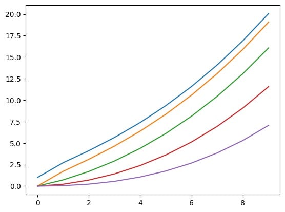
and looking at the weight distribution at a given time-step, this seems distributed exponentially.
Replies from: Stefan42, TurnTrout↑ comment by StefanHex (Stefan42) · 2023-06-25T12:29:38.483Z · LW(p) · GW(p)
Huh, thanks for this pointer! I had not read about NTK (Neural Tangent Kernel) before. What I understand you saying is something like SGD mainly affects weights the last layer, and the propagation down to each earlier layer is weakened by a factor, creating the exponential behaviour? This seems somewhat plausible though I don't know enough about NTK to make a stronger statement.
I don't understand the simulation you run (I'm not familiar with that equation, is this a common thing to do?) but are you saying the y levels of the 5 lines (simulating 5 layers) at the last time-step (finished training) should be exponentially increasing, from violet to red, green, orange, and blue? It doesn't look exponential by eye? Or are you thinking of the value as a function of x (training time)?
I appreciate your comment, and looking for mundane explanations though! This seems the kind of thing where I would later say "Oh of course"
↑ comment by Garrett Baker (D0TheMath) · 2023-06-27T04:17:58.166Z · LW(p) · GW(p)
You're right, that's not an exponential. I was wrong. I don't trust my toy model enough to be convinced my overall point is wrong. Unfortunately I don't have the time this week to run something more in-depth.
↑ comment by TurnTrout · 2023-06-26T17:53:46.526Z · LW(p) · GW(p)
So we should expect the first layer to have a larger norm than preceding layers.
you mean the final layer?
Replies from: D0TheMath↑ comment by Garrett Baker (D0TheMath) · 2023-06-27T04:16:39.539Z · LW(p) · GW(p)
Yes.
comment by Nate Showell · 2023-05-10T04:52:46.871Z · LW(p) · GW(p)
According to Stefan's experimental data, the Frobenius norm of a matrix is equivalent to the expectation value of the L2 vector norm of for a random vector (sampled from normal distribution and normalized to mean 0 and variance 1). So calculating the Frobenius norm seems equivalent to testing the behaviour on random inputs. Maybe this is a theorem?
I found a proof of this theorem: https://math.stackexchange.com/questions/2530533/expected-value-of-square-of-euclidean-norm-of-a-gaussian-random-vector
Replies from: Stefan42↑ comment by StefanHex (Stefan42) · 2023-05-10T11:30:43.396Z · LW(p) · GW(p)
Thanks for finding this!
There was one assumption in the StackExchange post I didn't immediately get, that the variance of is . But I just realized the proof for that is rather short: Assuming (the variance of ) is the identity then the left side is
and the right side is
so this works out. (The symbols are sums here.)
comment by Joseph Bloom (Jbloom) · 2023-05-07T01:38:01.084Z · LW(p) · GW(p)
I really liked this post and would like to engage with it more later. It could be very useful!
However, I also think that it would be good for you to add a section reviewing previous academic work on this topic (eg: https://aclanthology.org/2021.emnlp-main.133.pdf. This seems very relevant and may not be the only academic work on this topic (I did not search long). Curious to hear what you find!
Replies from: Stefan42↑ comment by StefanHex (Stefan42) · 2023-05-07T10:07:49.794Z · LW(p) · GW(p)
Thanks for the comment and linking that paper! I think this is about training dynamics though, norm growth as a function of checkpoint rather than layer index.
Generally I find basically no papers discussing the parameter or residual stream growth over layer number, all the similar-sounding papers seem to discuss parameter norms increasing as a function of epoch or checkpoint (training dynamics). I don't expect the scaling over epoch and layer number to be related?
Only this paper mentions layer number in this context, and the paper is about solving the vanishing gradient problem in Post-LN transformers. I don't think that problem applies to the Pre-LN architecture? (see the comment by Zach Furman for this discussion)
Replies from: Jbloom↑ comment by Joseph Bloom (Jbloom) · 2023-05-08T00:27:10.672Z · LW(p) · GW(p)
Thanks for the feedback. On a second reading of this post and the paper I linked and having read the paper you linked, my thoughts have developed significantly. A few points I'll make here before making a separate comment:
- The post I shared originally does indeed focus on dynamics but may have relevant general concepts in discussing the relationship between saturation and expressivity. However, it focuses on the QK circuit which is less relevant here.
- My gut feel is that true explanations of related formula should have non-trivial relationships. If you had a good explanation for why norms of parameters grew during training it should relate to why norms of parameters are different across the model. However, this is a high level argument and the content of your post does of course directly address a different phenomenon (residual stream norms). If this paper had studied the training dynamics of the residual stream norm, I think it would be very relevant.
