A circuit for Python docstrings in a 4-layer attention-only transformer
post by StefanHex (Stefan42), Jett Janiak (jett) · 2023-02-20T19:35:14.027Z · LW · GW · 8 commentsContents
  Introduction
    What are circuits
    How we chose the candidate task
    The docstring task
  Methods: Investigating the circuit
    Possible docstring algorithms
    Token notation
    Patching experiments
  Results: The Docstring Circuit
    Tracking the Flow of the answer token (C_def)
      Residual Stream patching
      Attention Head patching
    Tracking the Flow of the other definition tokens (A_def, B_def)
      Residual Stream Patching
      Attention Head patching
    Tracking the Flow of the docstring tokens (A_doc, B_doc)
      Residual Stream Patching
      Attention Head Patching
    Summarizing information flow
    Surprising discoveries
      Multi-Function Head 1.4
      Positional Information Head 0.4
      Duplicate Token Head 0.5 is mostly just transforming embeddings
      Duplicate Token Head 1.2 is helping Argument Movers
  Putting it all together
  Open questions & leads
None
8 comments
Produced as part of the SERI ML Alignment Theory Scholars Program under the supervision of Neel Nanda - Winter 2022 Cohort.
TL;DR: We found a circuit in a pre-trained 4-layer attention-only transformer language model. The circuit predicts repeated argument names in docstrings [? · GW] of Python functions, and it features
- 3 levels of composition,
- a multi-function head that does different things in different parts of the prompt,
- an attention head that derives positional information using the causal attention mask.
Epistemic Status: We believe that we have identified most of the core mechanics and information flow of this circuit. However our circuit only recovers up to half of the model performance [? · GW], and there are a bunch of leads [? · GW] we didn’t follow yet.

A_def, …) as well as (b) an actual prompt (load, …). The boxes show attention heads, arranged by layer and destination position, and the arrows indicate Q, K, or V-composition between heads or embeddings. We list three less-important heads at the bottom for better clarity.Introduction
Click here [? · GW] to skip to the results & explanation of this circuit.
What are circuits
What do we mean by circuits? A circuit in a neural network, is a small subset of model components and model weights that (a) accounts for a large fraction of a certain behavior and (b) corresponds to a human-interpretable algorithm. A focus of the field of mechanistic interpretability is finding and better understanding the phenomena of circuits, and recently the field has focused on circuits in transformer language models. Anthropic found the small and ubiquitous Induction Head circuit in various models, and a team at Redwood found the Indirect Object Identification (IOI) [LW · GW] circuit in GPT2-small.
How we chose the candidate task
We looked for interesting behaviors in a small, attention-only transformer with 4 layers, from Neel Nanda’s open source toy language models. It was trained on natural language and Python code. We scanned the code dataset for examples where the 4-layer model did much better than a similar 3 layer one, inspired by Neel's open problems [? · GW] list. Interestingly, despite the circuit seemingly requiring just 3 levels of composition, only the 4-layer model could do the task.
The docstring task
The clearest example we found was in Python docstrings, where it is possible to predict argument names in the docstring: In this randomly generated example, a function has the (randomly generated) arguments load, size, files, and last. The docstring convention here demands each line starting with :param followed by an argument name, and this is very predictable. Turns out that attn-only-4l is capable of this task, predicting the next token (files in the example shown here) correctly in ~75% of cases.

files. All argument names and descriptions are randomly sampled words. We've also looked into Google-style docstrings and found similar performance, but won't discuss this further here.Methods: Investigating the circuit
Possible docstring algorithms
There are multiple algorithms which could solve this task, such as
- "Docstring Induction": Always predict the argument that, in the definition, follows the argument seen in the previous docstring line. I.e. look for
param size, check the order in the definitionsize, files, and predictfilesaccordingly. - Line number based: In the Nth line predict the Nth variable from the definition, irrespective of the content of the other lines. I.e after the 3rd
paramtoken, predict the 3rd variablefiles. - Inhibition based: Predict variable names from the definition, but inhibit variable names which occurred twice (similar to the inhibition in the IOI circuit [AF · GW]), i.e. predict
load,size,files,last, and inhibit the former two. Add some preference for earlier tokens to preferfilesoverlast.
We are quite certain that at least the first two algorithms are implemented to some degree. This is surprising, since one of the two should be sufficient to perform the task; we do not investigate further why this is the case. A brief investigation showed that the implementation of the 2nd algorithm seems less robust and less generalizable that our model's implementation of the first one.
For this work we isolate and focus on the first algorithm. We do this by adding additional variable names to the definition such that the line number and inhibition based methods will no longer produce the right answer.
Original docstring (randomly generated example), with added arguments :

It's worth noting that on this task the model performs worse than on the original one. That is, it doesn't predict files as often and when it does it's less confident in its prediction. But it's a weird prompt with a less clear answer, so this is expected. The model will choose the "correct" answer files in 56% of the cases (significantly above chance!), the average logit diff is 0.5.
Token notation
Since our tokens are generated randomly we will just denote them as rand0, rand1 and so on, highlighting the relevant (repeated) variable names. For repeated tokens we add clarification after an underscore, i.e. whether the token is A in the definition (A_def) or docstring (A_doc), whether a comma follows A or B as ,_A or ,_B respectively, or whether we refer to the param token in line 1, 2 or 3 as param_1-3.
Token notation used for axes labels in this post:

A, B, C as well as rand tokens are randomly chosen words, but A_def and A_doc (B_def and B_doc) are the same random word. We disambiguate param and , tokens as param_1 and ,_A etc. so that e.g. the definition contains the tokens |A_def|,_A|B_def|. The special character · makes spaces visible.Patching experiments
Our main method for investigating this circuit is activation patching. That is, overwriting the activations of a model component -- e.g. the residual stream or certain attention head outputs -- with different values. This is also referred to as resampling-ablation [AF · GW], differing from zero or mean-ablation in that we replace the activations in one run with those from a different run, rather than setting them to a constant.
This allows us to run the model on a pair of prompts ("clean" and "corrupted"), say with different variable names, and replace some activations in the clean run with the corresponding activations from the corrupted run. Note that this corrupted --> clean patching is the opposite direction from the commonly used clean --> corrupted patching. Our method will show us whether these activations contained important information, if that information was different between the prompts.
We only investigate how the model knows to choose a correct variable name from all words (definition and docstring arguments) available in the context. We don't focus on how it knows that predicting any variable name (instead of tokens like def, ( ,, etc.) is a reasonable thing to do. To this extent we
- Choose the logit difference as our performance metric: We measure whether an intervention changes the difference between the logit of the correct answer
Cand the highest wrong-answer logit (maximum logit of all other definition and docstring argument names including corrupted variants, i.e.A,B,rand1,rand2, ..., maximum recalculated every time). - Patch only from what we call the "docstring distribution", corrupted prompts where we exchange argument names (highlighted in red) but leave the docstring frame (grey) intact. The three corrupted prompts we use are
- random answer: Replace the correct answer
C_defin the definition with a random word. - random def: Replace all arguments in the definition other than
C_def(i.e.A_defandB_def) with random words. This does not change the docstring argument valuesA_docorB_doc. - random doc: Replace all arguments in the docstring (i.e.
A_docandB_doc) with random words, without changing the definition.
- random answer: Replace the correct answer
Running a forward pass on these corrupted prompts gives us activations where some specific piece of information is missing. Patching with these activations allows us to track where this piece of information is used.
For all experiments and visualizations (patching, attention patterns) we use a batch of 50 prompts. For each prompt we randomly generate arguments (A, B, C) and filler tokens (rand0, rand1, ...).
Results: The Docstring Circuit
In this section we will go through the three components that make up our circuit and show how we identified each of them. Most of our findings are based on patching experiments, and in each of the following 3 subsections we will use one of the three corruptions. For each corruption, we first patch the residual stream to track the information flow between layers and token positions. Then we patch the output of every head at every position to understand how that information moves.
Tracking the Flow of the answer token (C_def)
The first step is to simply replace the token that should contain the answer (i.e. C in the definition) with a different token, and run the model with this "corrupted" prompt, saving all activations. These saved activations cannot have any information about the real original value of C_def (the only appearance of C in the prompt is replaced with a different random word in the corrupted run). Thus, when we do our patching experiments, i.e. overwrite a particular set of activations in a clean run with these corrupted activations, those activations will lose any information about the correct C_def value.
Residual Stream patching
You can see interactive versions of all of the plots in the Colab notebook.
Now for this first experiment, we patch (i.e. overwrite) the clean activations of residual stream before or after a certain layer and at a certain token position with the equivalent corrupted-run activations. We expect to see a negative change in logit difference anywhere the residual stream carries important information that is influenced by the C_def value.

C_def token value (the only information that is different in the corruption).- Concretely, we see that overwriting the residual stream before layer 0 at position
C_defdestroys performance -- this is expected since we just overwrite theC_defembedding and make it impossible for the remainder of the model to access the correctC_defvalue. - We also see an almost identical effect when overwriting before layer 1, 2 or 3 -- this shows us that the model still relies on the residual stream at this position containing the correct
C_defvalue. - Finally we see that overwriting the residual stream after layer 3 has only an effect at the last position
param_3. This is expected since the last layer only affects the logits, but it also shows us that after layer 3, the residual stream at theparam_3position contains important information about theC_defvalue.
Thus we can conclude that during layer 3 the model must have read the C_def information from the C_def token position and copied that information to the param_3 position.
Attention Head patching
Next we investigate which model component is responsible for this copying of information. We know it is one of the attention heads because our model is attention-only, but even aside from this only attention heads can move information between positions.
Rather than overwriting the residual stream, we overwrite just the output of one particular attention head. We overwrite the attention head's output with the output it would have had in a corrupted run, i.e. if it had not know the true value of C_def. We expect to see negative logit difference in all attention heads that write important information influenced by the C_def value.

C_def token, most significantly heads 3.0 and 3.6.Now we see for every attention head (denoted as layer.head) whether it carries important information about the answer value C_def, which is the corruption we use here.
Most strongly we see heads 3.0 and 3.6 -- these heads are writing information about the C_def value into the param_3 token position. From the previous plot we know that there must be heads in layer 3 that move information from the C_def position into the param_3 position, and the ones we found here are good candidates. We can confirm they are indeed reading the information from the C_def position by checking their (clean-run) attention pattern. Both heads attend to all argument names from destination param_3 , but about twice as much to C_def. This is consistent with positive, but quite low average logit difference of 0.5 on this task.

param_3. The heads clearly attend to the definition arguments, and most strongly to the correct answer C_def.Takeaway: Heads 3.0 and 3.6 move information from C_def to the final position param_3, and thus the final output logits. From now on we will call these the Argument Mover Heads, as they copy the name of the argument.
Side note: We can see a couple of other heads in the attention head patching plot. We don't think any of these are essential, so feel free to skip this part, but we'll briefly mention them. Head 2.3 seems to write a small amount of useful information into the final position as well, but upon inspection of its attention pattern it just attends to all definition variables without knowing which is the right answer. Furthermore, the output of a bunch of heads (0.0, 0.1, 0.5, 1.2, 2.2) writes information about the C_def value into the C_def position. We discuss the most significant ones (0.5 and 1.2) in separate sections at the end, but do not investigate the other heads in detail.
Tracking the Flow of the other definition tokens (A_def, B_def)
Now that we know where the model is producing the answer, we want to find out how it knows which is the right answer. Logically we know that it must be making use of the matching preceding arguments A and B in the definition and in the docstring to conclude which argument follows next.
Residual Stream Patching
We start by repeating our patching experiments, this time replacing the definition tokens A_def and B_def with random argument names. (We will cover docstring tokens in the next section.) First we patch the residual stream activations again, overwriting the activations in a clean run with those from a corrupted run, before or after a certain layer and at a certain position.

A_def and B_def were replaced by random words). Colored parts must depend on the corrupted information and affect the result.We focus on the most significant effects first:
- Before Layer 0: we see that before layer 0 (i.e. in the embeddings) patching the
B_deftoken destroys the performance. This makes sense as the model relies onB_defandB_docvalues matching, and without knowing the value ofB_defat all the model will perform badly. We also see a small effect of replacingA_def, but this is much weaker and tells us the model relies mostly onBrather thanAandB, so we will focus on theB_definformation from now on. - Between Layer 0 & Layer 1 we see that not much has changed during layer 0. The model still relies on the residual stream at position
B_defcontaining the information about the value ofB_defand breaks if we overwrite that position before layer 1. - Between Layer 1 & Layer 2 things get interesting: We see that the most important column, i.e. the position that contains the most important information about
B_defis the comma afterB_def(which we call,_B)! It is worth emphasizing here that theB_defposition will almost always contain information about theB_deftoken, even here and in later layers, but that is no longer relevant for the performance of the model. In layer 2, the model mostly relies on the,_Bposition to contain information aboutB_def. - Between Layer 2 & Layer 3 we see another change: The information moved again, and now only the residual stream at the
C_defposition is relevant for layer 3. This means that now only the residual stream activations of theC_defposition matter when it comes to differentiating between the clean and corruptedB_defvalues. - After Layer 3, as expected, only shows an effect in the param_3 position, as this is the only position influencing the prediction logits.
Side notes: Looking at the less significant effects we can see (i) that between layer 1 and 2 it is actually not only the ,_B position but also still the B_def position that is relevant. It seems these positions share a role here. And (ii) we notice that activations at positions A_doc and B_doc are affected by this A_def / B_def patch, we will see that this is related to duplicate token head 1.2 and discuss it later.
Attention Head patching
Now that we have seen how the information is moving from B_def to ,_B in layer 1, to C_def in layer 2, and finally to param_3 in layer 3 we want to find out which attention heads are responsible for this. Again we patch attention head outputs, overwriting the clean outputs with those from the corrupted run.

A_def and B_def where replace by random words. This shows us which heads' outputs into which positions are important and affected by A_def and B_def values.Focusing on the most significant effects again, we see exactly two heads match the criteria mentioned in the previous paragraph: Head 1.4 writes information into ,_B and head 2.0 writes into C_def.
We suspect that head 1.4 (writing into ,_B) thus reads this information from the B_def position. We can confirm this by looking at its attention pattern and see the head indeed strongly attends to B_def.

Similarly head 2.0 might be the head copying the information from ,_B to C_def in layer 2, and indeed its attention pattern strongly attends to ,_B.

In terms of mechanisms, these heads just seem to attend to their previous tokens. This is a common mechanism in transformers and can easily be implemented based on the positional embeddings, these heads are usually called Previous Token Heads. However since they do not only attend to the previous but the last couple of tokens, and sometimes the current token too, we will call these heads Fuzzy Previous Token Heads here.
Finally we see the heads 3.0 and 3.6 again. As we have already seen in the last attention head patching experiment, these Argument Mover Heads copy information from C_def into the final param_3 position, and also explain what we see in this attention head patching plot.
Takeaway: Heads 1.4 and 2.0 seem to be Fuzzy Previous Token Heads that move information about the value of the B_def token from the B_def position via the ,_B position to the C_def position.
Side notes: Again we see head 0.5 write B_def dependent information into the B_def position, similarly as we saw with C_def. We also see head 1.2 writing into the A_doc and B_doc positions as mentioned earlier. Both of these will be discussed at the end of this post. We also notice that patching head 2.2's output improves performance -- this is surprising, and reminds us of the "negative heads" found in the IOI paper, but we will leave this for a future investigation.
Tracking the Flow of the docstring tokens (A_doc, B_doc)
Our final set of experiments in this section is concerned with analyzing how the docstring is processed in the circuit. As mentioned in the previous section, we know that the model must be using this information, so in now section we want to see
- How the model locates the arguments
A_docandB_docin the docstring - How this influences the model in choosing
C_defas the final answer
Residual Stream Patching
We start again by looking at the residual stream patching plot for a rough orientation, before we dive into the attention head patching plot.

A_doc and B_doc were replaced by random words). Color shows effect of patching this part on the performance (logit difference).This looks relatively straightforward! Looking at the first row we see that the A_doc value isn't used at all so we ignore it again for the rest of this section -- only the value of B_doc matters. In terms of layers and positions that are important for the result and influenced by the B_doc patch, we see it is the B_doc position before layer 1, and the param_3 position after layer 1. This means the network does not care about the B_doc value in the B_doc position anymore after layer 1! It has read the information from there and no longer does anything task-relevant with this information at this position.
Let's look for this layer 1 head that copies B_doc-information into param_3 in the attention head patching plot.
Attention Head Patching

A_doc and B_doc where replace by random words. This shows us which heads' outputs are affected by A_doc and (more importantly) B_doc values.We immediately see head 1.4 writing into param_3, and its output must importantly depend on the value of B_doc since overwriting its activations with its corrupted version leads to a large change in logit difference. What is not clear is how head 1.4 is affected by the B_doc value. Looking at its attention pattern it is clear that the head is definitely attending to B_doc:

You might recognize this attention pattern as that of an Induction Head -- a head that attends to the token (B_doc) following a previous occurrence (param_2) of the current token (param_3) -- see this post [LW · GW] for a great explanation.
Side note: param_1 is another previous occurrence of the current token followed by A_doc, which is weakly attended to as well. Head's 1.4 attention prefers later induction targets, we'll show how it does it later (it's more complicated than you think!).
Induction heads rely on at least one additional head in the layer below, a Previous Token Head at the position the induction had is attending to (B_doc). This one won't show up in our patching plot since its output depends on param_2 only, so we ran a quick patching experiment replacing param_2 and scanned the attention patterns of layer 0 heads. We see that head 0.2 is important and has the right attention pattern, thus we believe it is the (Fuzzy) Previous Token Head for the induction subcircuit, but we are less confident in this.

Take away: We have found an induction circuit allowing head 1.4 to find the B_doc token and copy information about B into the param_3 position. From there, the Argument Mover Heads 3.0 and 3.6 use this to locate the answer.
Side notes: Less significant heads here are 0.5, 1.2, and 2.2. The former two will be discussed in later sections, and 2.2 (as mentioned in the previous section) won't be discussed further.
It's worth emphasizing that head 1.4 is acting as an Induction Head at this position, while it seemed to be acting like a Fuzzy Previous Tokens Head in the previous section -- from the evidence shown so far it's not clear that 1.4 isn't an Induction Head in both cases but in a dedicated section further down we will show that head 1.4 indeed behaves differently depending on the context!
Summarizing information flow
Summarizing our findings so far, we found that heads 1.4 and 2.0 act as Fuzzy Previous Tokens Heads and move information about B from B_def via ,_B to the C_def position, completing what we call the "def subcircuit".
We also found Fuzzy Previous Tokens Head 0.2 and Induction Head 1.4 moving information about B to the param_3 position; we call this the "doc subcircuit".
And finally we have the Argument Mover Heads 3.0 and 3.6 at position param_C whose outputs we have shown to depend on both B_def and B_doc, as well as the answer value C_def. It is using that B-information carried by the two subcircuits to attend from param_C to C_def and then copy the answer value from that position
We have illustrated all these processes in the diagram below, adding notes about Q, K and V composition as inferred from the heads behavior:

B information in the definition and docstring respectively, and the final argument mover heads which copy the right answer to the output.In the next sections we will cover (a) some surprising features of the circuit, as well as (b) some additional components that don't seem essential to the information flow but contribute to circuit performance.
Surprising discoveries
We encountered a couple of unexpected behaviors (head 1.4 having multiple functions, head 0.4 deriving position from causal mask) as well as a couple of heads with non-obvious functionality that we want to understand more deeply.
Multi-Function Head 1.4
Recall that the head 1.4 appears twice in our circuit. First, in the def subcircuit, acting as a Fuzzy Previous Token Head. Second, in the doc subcircuit, acting as an Induction Head.

,_B to the previous token B_def.
param_3 to B_doc that followed param_2.How does it do it? We investigated how much the behavior is dependent on the destination token.
Consider short prompts of the form |BOS|S0|A|B|C|S1|, where A, B and C are different words and S0 and S1 are the same "special" token. We would expect a pure Induction Head to always attend from S1 to A and a pure Previous Token Head to always attend from S1 to C. But for head 1.4 this behavior will vary depending on what we set as S0 and S1. The plot below shows exactly that.

|BOS|S0|A|B|C|S1|, where A, B and C are random words and S0 and S1 are the same "special" token.From setting the two special tokens to param, or to ⏎······ (newline with 6 spaces, which serves a similar role to param in a different docstring style) we see an induction-like pattern (1st and 2nd row respectively). For a , the attention is mostly focused on the current token and a few tokens back. For an = it's similar except with less attention to the current token. For most other words (e.g. lemon, oil) it only attends to BOS, which we interpret as being inactive.
Side note: We suspect that current token isn't even sufficient to judge the behavior. It turns out that in the prompt of the form |BOS|,|A|B|=|,| it seems to behave as an Induction Head, even though on |BOS|,|A|B|C|,| it's a Fuzzy Previous Token Head. We believe it's useful for dealing with default argument values like size=None, files="/home". It suggests the behavior is dependent on the wider context, not just on the destination token and probably involves some composition.
Positional Information Head 0.4
We didn't know how the head 1.4 attends much more to B_doc than to A_doc. If it was following a simple induction mechanism, then it should attend equally to both as they both follow a param token.
The obvious solution would be to make use of the positional embedding and attend more to recent tokens. However, when we swap the positional embeddings of A_doc and B_doc before we feed them to 1.4, it doesn't change the attention pattern significantly. We also tested variations of this swap, such as swapping positional embeddings of the whole line, or accounting for layer 0 head outputs leaking positional embeddings, with similar results.
The other source of positional information is the causal mask. We see that head 0.4 has an approximately constant attention score, and thus the attention pattern decreases with destination position, similar to what Neel Nanda found (video) in a model trained without positional embeddings.

BOS (left column) is by far the most significant, and decreases the larger the distance between the destination position and BOS.Our hypothesis is that head 0.4 provides the positional information for head 1.4 about which argument (A_doc vs B_doc) is in the most recent line, and thus correct to attend to. Testing this we plot 1.4's attention pattern for four cases: (i) the baseline clean run, and for runs where we swap (i) the positional embeddings of A_doc and B_doc, (ii) the attention pattern of head 0.4 at A_doc and B_doc destination position, or (iii) both. We conclude that, indeed, the decisive factor for head 1.4 seems to be head 0.4's attention pattern.

A_doc and B_doc (from destination param_3). This is evidence that the causal attention mask in head 0.4 provides positional information that head 1.4 uses to attend to the most recent docstring line. Swapping head 0.4's attention pattern inverts 1.4's attention, while swapping the positional embedding barely affects it.Duplicate Token Head 0.5 is mostly just transforming embeddings
Head 0.5 is important for the docstring task at positions B_def, C_def, and B_doc (up to 1.1 logit diff change). But its role can be almost entirely explained as transforming the embedding of the current token. In fact, setting its attention pattern to an identity matrix for the whole prompt loses less than 0.1 logit diff.
This embedding transformation explains why head 0.5 shows up in most of our patching plots. We also expect most heads that compose with the embeddings to appear as composing with 0.5.
More generally, we expect the model to rely on the fact that head 0.5's output -- besides some positional information -- only depends on the token embedding of the current token (since any duplicate token has the same token embedding). Thus any methods looking at direct connections between heads and token embeddings may have to incorporate effects from heads like this.
The remaining 0.1 logit diff from diagonalizing head 0.5's attention comes mostly (~74%) from the attention pattern at destination B_doc and K-composition with Head 1.4. We discuss these details in the notebook, but don't focus on it here since (a) the effect is small and (b) does largely disappear if we ablate all the heads we believe not to be part of our circuit.
Duplicate Token Head 1.2 is helping Argument Movers
We noticed another Duplicate Token Head, 1.2. This head attends to the current token X_doc, previous occurrence X_def (where X is either A or B), and the BOS token if the destination is a docstring argument. If the destination is a definition argument it only attends to X_def or BOS.
We varied head 1.2's attention pattern between BOS, X_def, and X_doc and notice that only the amount of attention to BOS matters for performance.
Furthermore, based on our patching composition scores[1] we observed that head 1.2 composes with the Argument Mover Heads 3.0 and 3.6 (both heads behave similarly). So 1.2 must influence 3.0 and 3.6's attention patterns.
To analyze what it is doing we look at 3.0's attention pattern (destination param_3) as a function of 1.2's attention pattern (destination B_doc). We already know that the only relevant variable is how much head 1.2 attends to BOS so we vary this in the plot below:

B_doc. We found that attention to source BOS matters so we show 3.0's baseline attention pattern in the top panel, the relative change as a function of 1.2's BOS-attention in the bottom panel.The baseline attention pattern of head 3.0 is attending mostly to definition arguments, but with a small bump at B_doc. We observe that varying 1.2's attention to BOS changes the size of this bump! So we think that head 1.2 is used to suppress the Argument Mover Heads' attention to docstring tokens and thus improves circuit performance by predicting the wrong B answer (via B_doc) less often.
Our explanation for this, i.e. for why head 1.2's attention to BOS (color in plot) is higher in the definition, is the following: In the docstring (as shown here) the head encounters arguments X (where X is A or B) as repeated tokens, so its attention is split between BOS, X_def, and X_doc and thus attends less to BOS. In the definition, its attention is only split between BOS and X_def and thus attends more to BOS.
This argument makes sense, and it is plausible that this is the reason for the improved performance. However we should note that this "small bump" is a relatively small issue, and the total effect of this head at A_doc or B_doc (compared to the corrupted version) is only a logit difference change of -0.12. The change at A_def or B_def is +0.05, and -0.20 at C_def. This matches with our hypothesis that head 1.2 increases attention to definition arguments, and decreases attention to docstring arguments.
Putting it all together
Now we have a solid hypothesis which heads are involved in the circuit, mainly heads 1.4, 2.0, 3.0, and 3.6 for moving the information, head 0.5 for token transformation and some additional support, as well as 1.2 for additional support.
At least Previous Token Head 0.2 and Positional Information Head 0.4 (and potentially more) are also essential parts of the circuit, but won't show differ in our patching experiments. To find these and any further heads we would need to expand to a non-docstring prompt distribution, but that's not our focus here.
Our final check to test whether this circuit is sufficient for the task is to patch (i.e. resample-ablate) all other heads and see if we recover the full performance. Note that we could expand this to take into account the heads position and composition (e.g. with causal scrubbing) but stick to the more coarse-grained check for now.
Testing the circuit performance with only this set of heads (0.2, 0.4, 0.5, 1.2, 1.4, 2.0, 3.0, 3.6) we get a success rate for predicting the right argument of 42% (chance is 17%).
The full model for comparison achieves 56%, and slightly augmenting the full model by removing heads 0.0 and 2.2 gave 72%.
We found that there is one large improvement to our circuit, adding head 1.0 brings performance to 48%, and also adding heads 0.1 and 2.3 brings performance to 58%. Beyond this point we found only small performance gains per head.
Open questions & leads
We believe we have understood most of the basic circuit components and what they do, but there are still details we want to investigate in the future.
- How exactly does attention head 1.4 implement different functions in different contexts? Is this a common theme in transformers?
- We're currently looking into this, and would love to collaborate!
- Test universality of this circuit across similar models
- We had some initial success finding similar circuits in similarly-sized 3- and 4-layer models with MLPs, we'd be interesting in collaborating on this!
- Follow leads on additional heads:
- Duplicate Token Head 0.1 seems to behave somewhat similar to head 1.2, but we don't understand its behaviour yet.
- Head 1.0 seems to be another Fuzzy Previous Token Head (similar to 1.4) but only relevant when restricting the model to the smaller set of heads in our circuit. Maybe some sort of Duplicate Token Head?
- Head 2.2 seems to be some sort of negative head, patching it with corruptions increases performance.
- Head 2.3 again seems to be only relevant when restricting the model to the smaller set of heads in our circuit. It seems to attend to all definition arguments equally, an avenue here would be checking a corruption that swaps
C_defwith e.g.rand2and see if patching 2.3's output has an effect (Thanks to Neel for the idea!)
- Testing the circuit more thoroughly, i.e. check also the composition and not just confirm the list of heads involved.
- Run the model with only the compositions allowed by the circuit, and all other connections resample-ablated. We would like to implement this in TransformerLens, collaborators welcome!
- Even more specifically, test the hypothesis with Causal Scrubbing [LW · GW].
Summary: We found a circuit that determines argument names in Python docstrings. We selected this behaviour because a 4-layer attention-only toy model could do the task while a 3-layer one could not. We "reverse engineered" the behaviour and showed that the circuit relies on 3 levels of composition. We find several features we have not seen before in this context, such as a multi-function attention head and an attention head deriving positional information using the causal attention mask. We also notice a large number of non-crucial mechanisms that improve performance by small amounts. We also found motifs seen in other works such as our Argument Mover heads that resemble the Name Mover heads found in the IOI paper.
Accompanying Colab notebook with all interactive plots is here.
Acknowledgements: Neel Nanda substantially supported us throughout the SERIMATS program and gave very helpful feedback on our research and this draft. Furthermore Arthur Conmy, Aryan Bhatt, Eric Purdy, Marius Hobbhahn, Wes Gurnee provided valuable feedback on research ideas and the draft.
This project would not have been possible without extensive use of TransformerLens, as well as the CircuitsVis and PySvelte.
- ^
We use a new kind of composition score based on patching (point-to-point resampling ablation): Composition between head Top and head Bottom is "How much does Top's output meaningfully change when we feed it the corrupted rather than clean output of Bottom?". We plan to expand on this in a separate post, but happy to discuss!
8 comments
Comments sorted by top scores.
comment by cmathw · 2023-05-12T08:27:25.316Z · LW(p) · GW(p)
This is really interesting work and is presented in a way that makes it really useful for others to apply these methods to other tasks. A couple of quick questions:
- In this work, you take a clean run and patch over a specific activation from a corresponding corrupt run. If you had done this the other way around (ie. take a corrupt run and see which clean run activations nudge the model closer to the correct answer), do you think that one would find similar results? Do you think there should be a preference to the whether one patches clean --> corrupt or corrupt --> clean?
- Did you find that the corrupt dataset that you used to patch activations had a noticeable effect on the heads that appeared to be most relevant? Concretely, in the 'random answer' corrupt prompt (ie. replacing the correct answer C_def in the definition with a random word), did you find that the selection of this word mattered (ie. do you expect that selecting a word that would commonly be found in a function definition be superior to other random words in the model's vocab) or were results pretty consistent regardless?
↑ comment by StefanHex (Stefan42) · 2023-05-25T11:58:11.137Z · LW(p) · GW(p)
Hi, and thanks for the comment!
Do you think there should be a preference to the whether one patches clean --> corrupt or corrupt --> clean?
Both of these show slightly different things. Imagine an "AND circuit" where the result is only correct if two attention heads are clean. If you patch clean->corrupt (inserting a clean attention head activation into a corrupt prompt) you will not find this; but you do if you patch corrupt->clean. However the opposite applies for a kind of "OR circuit". I historically had more success with corrupt->clean so I teach this as the default, however Neel Nanda's tutorials usually start the other way around, and really you should check both. We basically ran all plots with both patching directions and later picked the ones that contained all the information.
did you find that the selection of [the corrupt words] mattered?
Yes! We tried to select equivalent words to not pick up on properties of the words, but in fact there was an example where we got confused by this: We at some point wanted to patch param and naively replaced it with arg, not realizing that param is treated specially! Here is a plot of head 0.2's attention pattern; it behaves differently for certain tokens. Another example is the self token: It is treated very differently to the variable name tokens.
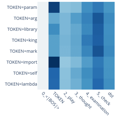
So it definitely matters. If you want to focus on a specific behavior you probably want to pick equivalent tokens to avoid mixing in other effects into your analysis.
comment by LawrenceC (LawChan) · 2023-02-20T20:42:22.076Z · LW(p) · GW(p)
Cool work, thanks for writing it up and posting!
We selected this behaviour because a 4-layer attention-only toy model could do the task while a 3-layer one could not.
I'm a bit confused why this happens, if the circuit only "needs" three layers of composition. Relatedly, do you have thoughts on why head 1.4 implements both the induction behavior and the fuzzy previous token behavior?
Replies from: Stefan42, neel-nanda-1↑ comment by StefanHex (Stefan42) · 2023-02-20T21:38:22.448Z · LW(p) · GW(p)
Yep, it seems to be a coincidence that only the 4-layer model learned this and the 3-layer one did not. As Neel said I would expect the 3-layer model to learn it if you give it more width / more heads.
We also later checked networks with MLPs, and turns out the 3-layer gelu models (same properties except for MLPs) can do the task just fine.
↑ comment by Neel Nanda (neel-nanda-1) · 2023-02-20T21:18:09.531Z · LW(p) · GW(p)
I'm a bit confused why this happens, if the circuit only "needs" three layers of composition
I trained these models on only 22B tokens, of which only about 4B was Python code, and their residual stream has width 512. It totally wouldn't surprise me if it just didn';t have enough data or capacity in 3L, even though it was technically capable.
Replies from: LawChan↑ comment by LawrenceC (LawChan) · 2023-02-20T21:31:06.017Z · LW(p) · GW(p)
Ah, that makes sense!
comment by Thomas Kwa (thomas-kwa) · 2024-05-08T03:09:42.257Z · LW(p) · GW(p)
The model ultimately predicts the token two positions after B_def. Do we know why it doesn't also predict the token two after B_doc? This isn't obvious from the diagram; maybe there is some way for the induction head or arg copying head to either behave differently at different positions, or suppress the information from B_doc.
Replies from: Stefan42↑ comment by StefanHex (Stefan42) · 2024-05-08T10:52:32.511Z · LW(p) · GW(p)
Thanks for the question! This is not something we have included in our distribution, so I think our patching experiments aren't answering that question. If I would speculate though, I'd suggest
- The Prev Tok head 1.4 might "check" for a signature of "I am inside a function definition" (maybe a L0 head that attends to the
defkeyword. This would make it work only on B_def not B_dec - Duplicate Tok head 1.2 might help the mover heads by suppressing their attention to repeated tokens. We observed this ("Duplicate Token Head 1.2 is helping Argument Movers"), but were not confident whether it is important. When doing ACDC we felt 1.2 wasn't actually too important (IIRC) but again this would depend on the distribution
In summary, I can think of a range of possible mechanisms how the model could achieve that, but our experiments don't test for that (because copying the 2nd token after B_dec would be equally bad for the clean and corrupted prompts).