Distilling the Internal Model Principle

post by JoseFaustino · 2025-02-08T14:59:29.730Z · LW · GW · 0 comments

Contents

  Overview
    Post Outline
  Introduction
  A simplified Internal Model Theorem
    Example 1: even-odd integer walking
  Equivalence relations as information
  Observability Condition
    Example 2 - Dyadic transformation
  Lemma: Generalized Feedback Condition
  The theorem
    Theorem: Internal Model Principle simplified
  The need to generalize
None
No comments

This post was written during the agent foundations fellowship with Alex Altair [LW · GW] funded by the LTFF. Thank you Alex Altair [LW · GW], Alfred Harwood [LW · GW] and Dalcy [LW · GW] for thoughts and comments.

Overview

This is the first part of a two-post series about the Internal Model Principle (IMP)^[1], which could be considered a selection theorem [LW · GW], and how it might relate to AI Safety, particularly to Agent Foundations research. 

In this first post, we will construct a simplified version of IMP that is easier to explain compared to the more general version and focus on the key ideas, building intuitions about the theorem's assumptions.

In the second post, we generalize the theorem and discuss how it relates to alignment-relevant questions such as the agent-structure problem [LW · GW] and selection theorems [LW · GW].

Post Outline

• We discuss the basic mathematical objects framed in a friendly-AI-tracking-a-super-AI setup and a condition called the "feedback structure condition".
  • With the basic setup and feedback condition, we're already able to construct a (not very useful) notion of an internal model.
• We digress about why equivalence relations represent information structure and how that can be used to specify the observability condition. These ideas are used to make the notion of the model better.
• We prove our particular version of the theorem - which requires quite strong assumptions. We end up with a notion of model, in some sense, doesn't seem very useful either.
  • This serves as motivation for why we need to generalize the assumptions in the second post.

Introduction

This section aims to explain the motivation for the post. Statements here might not be fully explained and will become clearer throughout the post. I aimed to include all the definitions and state mathematical facts used without proof to build the theorem from zero. Although there are a lot of equations in the post, there is little mathematical machinery used in the theorem. We mostly use facts about arbitrary functions and sets. I expect that someone with high-school level math could be able to understand this post if read carefully.

The Internal Model Theorem by Cai & Wonham ^[1] is an abstraction and generalization of the Internal Model Principle that appears in control theory examples. It's built directly on straightforward algebraic tools and a little bit of dynamical systems theory.

The theorem basically states: consider a discrete and deterministic external system passing signals to an internal system which can change its own states. If these signals satisfy a property we call "observability", which ensures that the internal system has enough precision about the receiving signal, then feedback structure and perfect regulation implies that the internal system necessarily has an internal model of the external system. 

Intuitively, "feedback" means that the internal system's output can be fed back into the internal system to produce the next output. "Feedback structure" is the condition that ensures this, i.e, that the internal system's state depends only on its previous state. It's autonomous - as opposed to "pursuing the states of the external system one time-step later"

"Perfect regulation" here means that the set of external system states are all good states, in some sense of good. Good states could be, for example, states where the "error" between the external system and internal system is zero, which we expect to happen after the external system has reached some sort of equilibrium or stationary state.

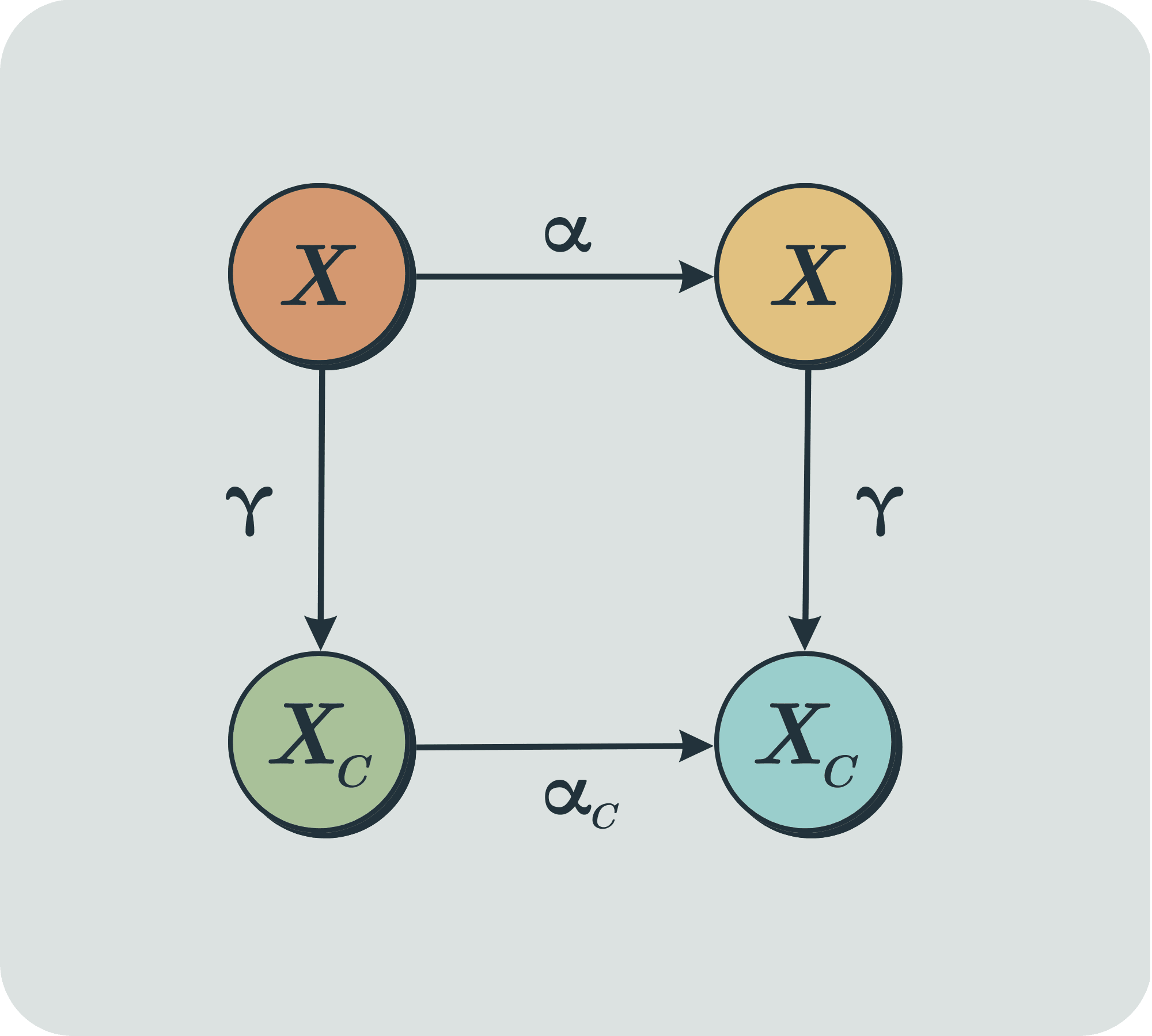
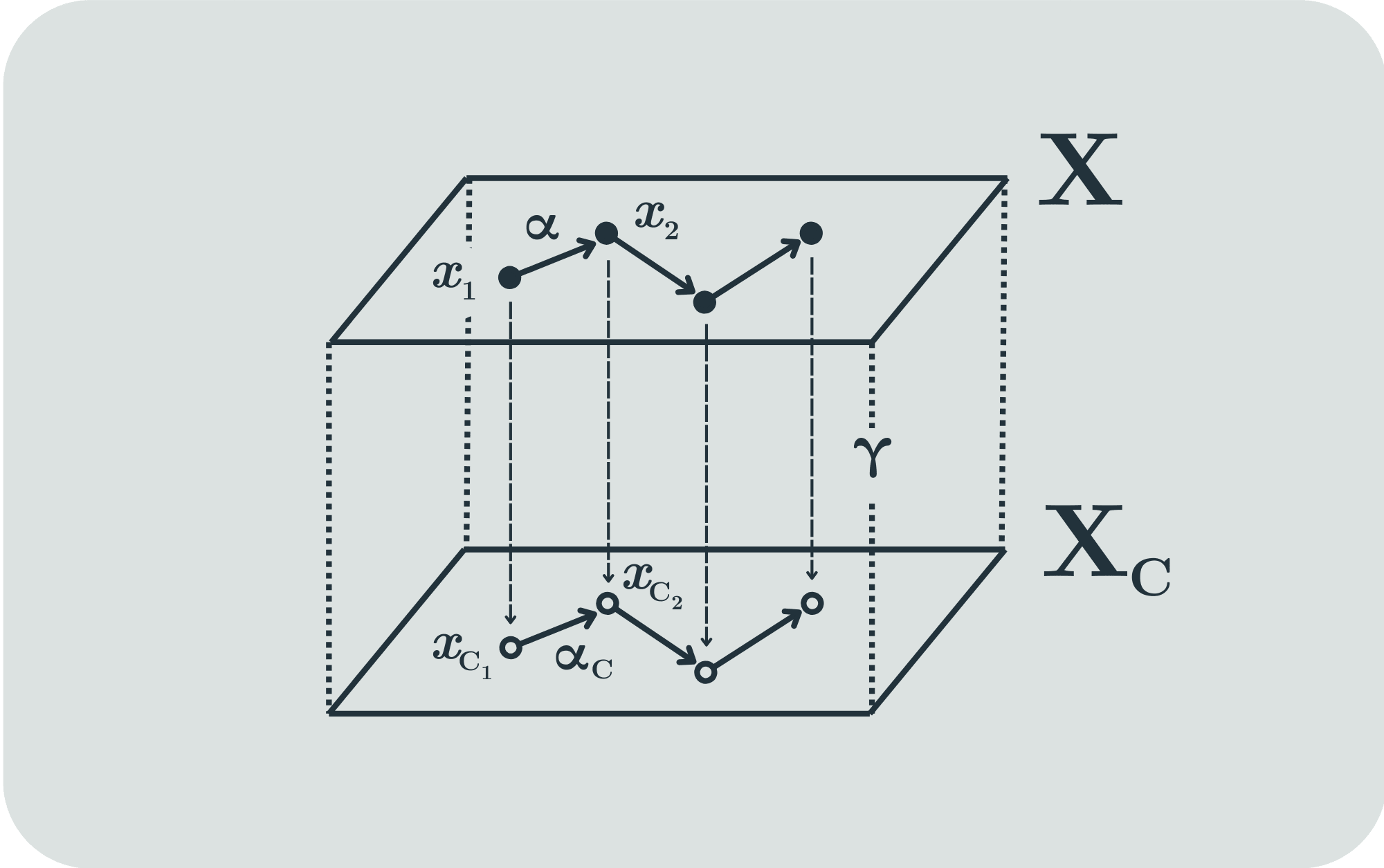
"Modeling" means "faithful tracking/simulating": we say system $A$ with dynamics ${\alpha }_A:X_A\to X_A$ models a system $B$ with dynamics ${\alpha }_B:X_B\to X_B$, where $A$ receives info from $B$ via $\gamma :X_B\to X_A$, if ${\alpha }_A\circ \gamma =\gamma \circ {\alpha }_B$ and $\gamma$ is injective.

• ${\alpha }_A\circ \gamma =\gamma \circ {\alpha }_B$ ensures simulation: Given a state $x\in X_B$, the information $A$ receives from ${\alpha }_B\left(x\right)$ is $\gamma \left({\alpha }_B\right(x\left)\right)$. The state the internal system is in after its own internal update is ${\alpha }_A\left(\gamma \right(x\left)\right)$. We're saying $A$ models $B$ if those are the same.
• $\gamma$ being injective ensures the notion of model is non-trivial, i.e, that A faithfully simulates B.  As we'll see later, if $\gamma$ is not injective, system A might not be expressive enough to model system B.

To illustrate, $A$ could be a robot trying to pursue a moving target $B$ in a controlled environment.

A simplified Internal Model Theorem

Suppose we have a very powerful and capable AI (which we'll refer to as ASI) and we don't have a clue about how it works, what decisions it makes, how it chooses these decisions, etc. One idea to understand its behavior is to make a friendly AI (FAI for short) oversee the ASI.

This is generally called "scalable oversight" in the AI Safety community, and we will use this idea to motivate the theorem. Don't get too caught up in the analogy, though - the theorem has strong assumptions that aren't necessarily satisfied in real settings. However, perhaps this theorem could be a good starting point to formulate better theories.

The ASI could be physical, virtual or any type of machine at all, and we would say that the ASI is in different states when its configuration is substantially different. For example, if the ASI is recharging its battery, we could say its state is $r$; if it is active, its state is $a$. If it's learning, we'd say its state is $l$; if it's inferring, we'd say its state is $i$.

Abstractly, we will call the ASI's internal state set $X$ and the rule that describes how its internal state changes $\alpha :X\to X$ . That is, if the ASI is in the state $x$, after one time-step, it will be in state $\alpha \left(x\right)$, then in $\alpha \left(\alpha \right(x\left)\right)$ and so on. We call update rules like these discrete dynamics. 

We assume the FAI has access to information about the ASI via a map $\gamma :X\to X_C$, where $X_C$ is the FAI state set (we call it $X_C$ because often in control theory this is called the “controller”) and we ask $\gamma \left(X\right)$ - the image of $X$ under $\gamma$ - to be equal to $X_C$ . This is not that big of a deal - we're only asking that any given state of the FAI represent information about some state of the ASI. If this was not the case, we could just change the co-domain of $\gamma$ to be $\gamma \left(X\right)$. Formally, this means that for every FAI state, it can be written as $x_C=\gamma \left(x\right)$ for some ASI state $x$. Thus, we can think that $\gamma$ defines $X_C=\gamma \left(X\right)$.

We want the FAI to track/predict/model the ASI, i.e, to simulate its behaviour in some intuitive sense. Since we can interpret the FAI, this might give us clues about the ASI's behaviour. 

We want, then, to model the FAI as a dynamical system on its own, i.e, one that autonomously evolves.  Otherwise, the FAI wouldn't be properly tracking/predicting the ASI's states. In other words, we want the FAI state $x_C=\gamma \left(x\right)$ to determine the next FAI state $x_C^{\prime }=\gamma \left(\alpha \right(x\left)\right)$. Equivalently, this is to say that if $x,y$ are ASI states such that $\gamma \left(x\right)=\gamma \left(y\right)$, then necessarily $\gamma \left(\alpha \right(x\left)\right)=\gamma \left(\alpha \right(y\left)\right)$, because $x_C^{\prime }=\gamma \left(\alpha \right(x\left)\right)=\gamma \left(\alpha \right(y\left)\right)$ can only depend on $x_C=\gamma \left(x\right)=\gamma \left(y\right)$

We call this the feedback structure condition, because it ensures that the next FAI state is just the feedback of the previous state. We will put a lot of emphasis on this because it's a fundamental hypothesis for the theorem. 

Now, some algebraic remarks to help any unfamiliar readers:

• We call the set of equivalence relations $E\left(X\right)$ and for $E_1,E_2$ equivalence relations on $X$, we say $E_1\le E_2⟺E_1\subseteq E_2$
  • One can also prove that every subset $A$ of $E\left(X\right)$ has an infimum and supremum, $inf\left(A\right),sup\left(A\right)\in E\left(X\right)$, with respect to the $\le$ ordering defined above
    • In particular, it’s true that $inf\left(A\right)={\bigcap }_{A\in A}A$ 
• Every equivalence relation $E\in E\left(X\right)$ generates a partition on $X$ - the partition $P=\left\{\right[x]\subset X;x\in X\},\text{where}\left[x\right]:=\{y\in X;(x,y)\in E\}$. Reciprocally, every partition $P$ of $X$ generates an equivalence relation on $X$, i.e, the equivalence relation such that two elements are related if and only if they’re in the same set of the partition. Thus, we can think of equivalence relations and partitions as the same thing
  • We call the sets $\left[x\right]$ cells
• If $f:X\to Y$ is any function, we define $\ker f:=\left\{\right(x,y)\in X\times X;f(x)=f(y\left)\right\}$ ^[2]
  • One can prove that $\ker f$ is an equivalence relation on X

Thus, we can rewrite the feedback condition as 

$$\ker \gamma \le \ker \gamma \circ \alpha$$

Which is the same as

$$\forall x,y\in X,(x,y)\in \ker \gamma ⟹\left(\alpha \right(x),\alpha (y\left)\right)\in \ker \gamma$$

This leads us to another way to think about the feedback condition: it's ensuring that two points that are in the same set of the partition induced by $\ker \gamma$ remain in the same (that is possibly different from the initial) partition set after the ASI updates. Intuitively, this is saying that the observations the FAI receives are consistent: two different ASI states $x,y$, that provide the same information to the FAI - $\gamma \left(x\right)=\gamma \left(y\right)$, can't provide two different pieces of information - $\gamma \left(\alpha \right(x\left)\right)\text{and}\gamma \left(\alpha \right(y\left)\right)$ - to the FAI after the ASI updates.

Framed differently, if we don't assume the feedback condition, we would be saying that two states that provide the same information to the FAI will provide different information after one time-step. Intuitively, if this were the case, it seems that the FAI wouldn't be able to track ASI's states at all.

We will prove later that this condition actually ensures that the information the FAI receives from the ASI remains consistent after any number of time-steps.

The basic setup and feedback condition discussed so far are enough for us to define a rule ${\alpha }_C:X_C\to X_C$ - called the FAI dynamics - that tracks the ASI: 

• Let $x_C\in X_C$, there is $x\in X$ such that $\gamma \left(x\right)=x_C$. Define ${\alpha }_C\left(x_C\right)=\gamma \left(\alpha \right(x\left)\right)$
  • Note that this definition is unambiguous: if $x^{\prime }\in X$ is such that $\gamma \left(x^{\prime }\right)=x_C$, then by the feedback condition, $\gamma \left(\alpha \right(x\left)\right)=\gamma \left(\alpha \right(x^{\prime }\left)\right)$
• Note that ${\alpha }_C\circ \gamma =\gamma \circ \alpha$
  • This is trivially the case by the definition of ${\alpha }_C$:
    • For all $x\in X,{\alpha }_C\left(\gamma \right(x\left)\right)=\gamma \left(\alpha \right(x\left)\right)$
  • We interpret this result as follows: for a given ASI state $x\in X$, the FAI's observation from the next state of the ASI is $\gamma \left(\alpha \right(x\left)\right)$. On the other hand, the FAI's update based on the current state observation is ${\alpha }_C\left(\gamma \right(x\left)\right)$. The result states those are the same: that is, the FAI's state after its own update having observed the current state is the same as the FAI's state observed from the ASI's state update. In other words, the FAI's state after an update corresponds to the observation of the ASI's state after the update.
• It's also true that ${\alpha }_C$ is unique: it is the only map ${\alpha }_C:X_C\to X_C$ such that ${\alpha }_C\circ \gamma =\gamma \circ \alpha$
  • Assume ${\alpha }_{C,1},{\alpha }_{C,2}\text{satisfy}{\alpha }_{C,i}\circ \gamma =\gamma \circ \alpha$. Then let $x_C=\gamma \left(x\right)\in X_C,{\alpha }_{C,1}\left(x_C\right)={\alpha }_{C,1}\left(\gamma \right(x\left)\right)=\gamma \left(\alpha \right(x\left)\right)={\alpha }_{C,2}\left(\gamma \right(x\left)\right)={\alpha }_{C,2}\left(x_C\right)$

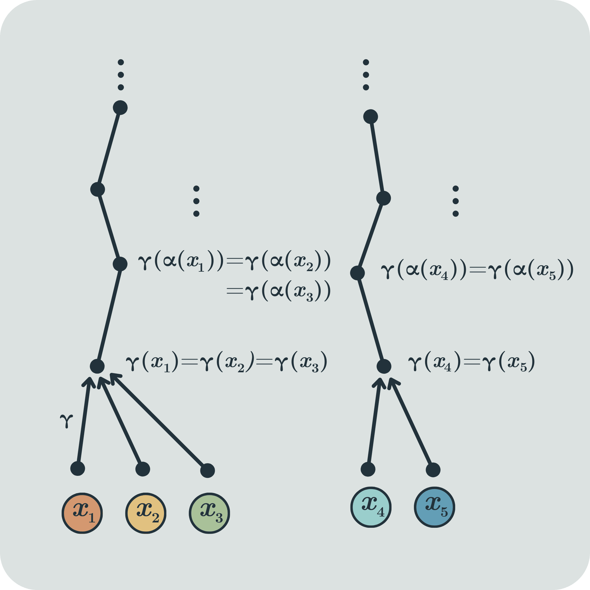
Example 1: even-odd integer walking

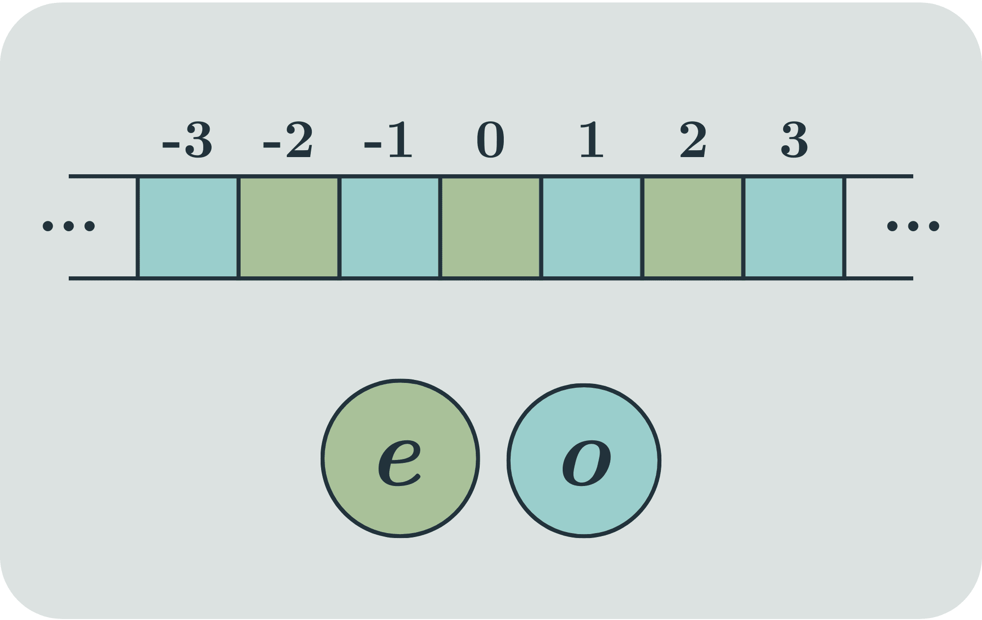
Consider a robot walking along the integers. It walks one unit to the right at each step, so its state set is $X=Z$ and its dynamics given by $\alpha :Z\to Z,\alpha \left(n\right)=n+1$, for all $n\in Z$.

Let $X_C=\{e,o\}$ and $\gamma :X\to X_C$ given by $\gamma \left(n\right)=e$ if $n$ is even and $\gamma \left(n\right)=o$ if $n$ is odd.

 

Since $\gamma \left(n_1\right)=\gamma \left(n_2\right)$ if, and only if $n_1\equiv n_2\left(\mathrm{mod}2\right)$, we have

$$\ker \left(\gamma \right)=\left\{\right(n_1,n_2)\in Z\times Z\mid n_1\equiv n_2(\mathrm{mod}2\left)\right\}$$

And 

$$\ker (\gamma \circ \alpha )=\left\{\right(n_1,n_2)\in Z\times Z\mid (n_1+1)\equiv (n_2+1\left)\right(\mathrm{mod}2\left)\right\}$$

We're allowed to add and subtract one on both sides of the integer congruence, hence $\ker \gamma =\ker \gamma \circ \alpha$, so the feedback condition holds. Hence, by the result proved above, ${\alpha }_C:X_C\to X_C$ exists and is uniquely determined by ${\alpha }_C\circ \gamma =\gamma \circ \alpha$

Now, calculating ${\alpha }_C$: 

• For $n$ even, ${\alpha }_C\left(e\right)={\alpha }_C\left(\gamma \right(n\left)\right)=\gamma \left(\alpha \right(n\left)\right)=\gamma (n+1)=o$
• For $n$ odd, ${\alpha }_C\left(o\right)={\alpha }_C\left(\gamma \right(n\left)\right)=\gamma \left(\alpha \right(n\left)\right)=e$

Thus, ${\alpha }_C$ autonomously alternates between states $e$ and $o$

We generally call $(X_C,{\alpha }_C)$ the "controller" for control theory reasons. We'll touch on that later.

It looks like the dynamic ${\alpha }_C$ of the controller is simulating the dynamics $\alpha$ of the robot, in some weak sense, but it doesn't feel like the controller is doing a very accurate simulation of the robot's behaviour - the controller can simulate the fact that the robot alternates between even- and odd-numbered positions, but it doesn't simulate the fact that the robot is moving indefinitely to the right. Ideally, we would want it to simulate both.

Can we add more assumptions to ensure that the controller accurately simulates the robot?

Since $X_C=\{e,o\}$, a dynamics ${\alpha }_C$ defined on $X_C$ can’t represent a trajectory more complicated than some sequence of states $e$ and $o$. Recall that $\gamma \left(X\right)=X_C$. Hence, to get a better notion of the model, we need to consider more assumptions about $\gamma$ (and thus $X_C$, if we think $X_C$ is defined by $\gamma \left(X\right)$). We can think that the controller states don't have enough "expressivity" to represent a model of the robot.

Another way to think about this is: if the observations that the FAI receives - which here are also the FAI's states - don’t encompass core information from the ASI's states, the FAI couldn’t possibly simulate the ASI.

Equivalence relations as information

We can interpret equivalence relations in $E\left(X\right)$ as information structures on $X$. Let $E\in E\left(X\right)$ and suppose an element $y\in X$ is ‘known exactly’. Recall that $E$ induces a partition on $X$, and that we call the sets forming the partition ‘cells’. Now, if $x\in X$ is such that $(x,y)\in E$, all the ‘information’ or ‘precision’ we know about $x$ is no more than that it is in the cell that contains $y$.

 Cai &Wonham ^[1]illustrates this idea with the following example:

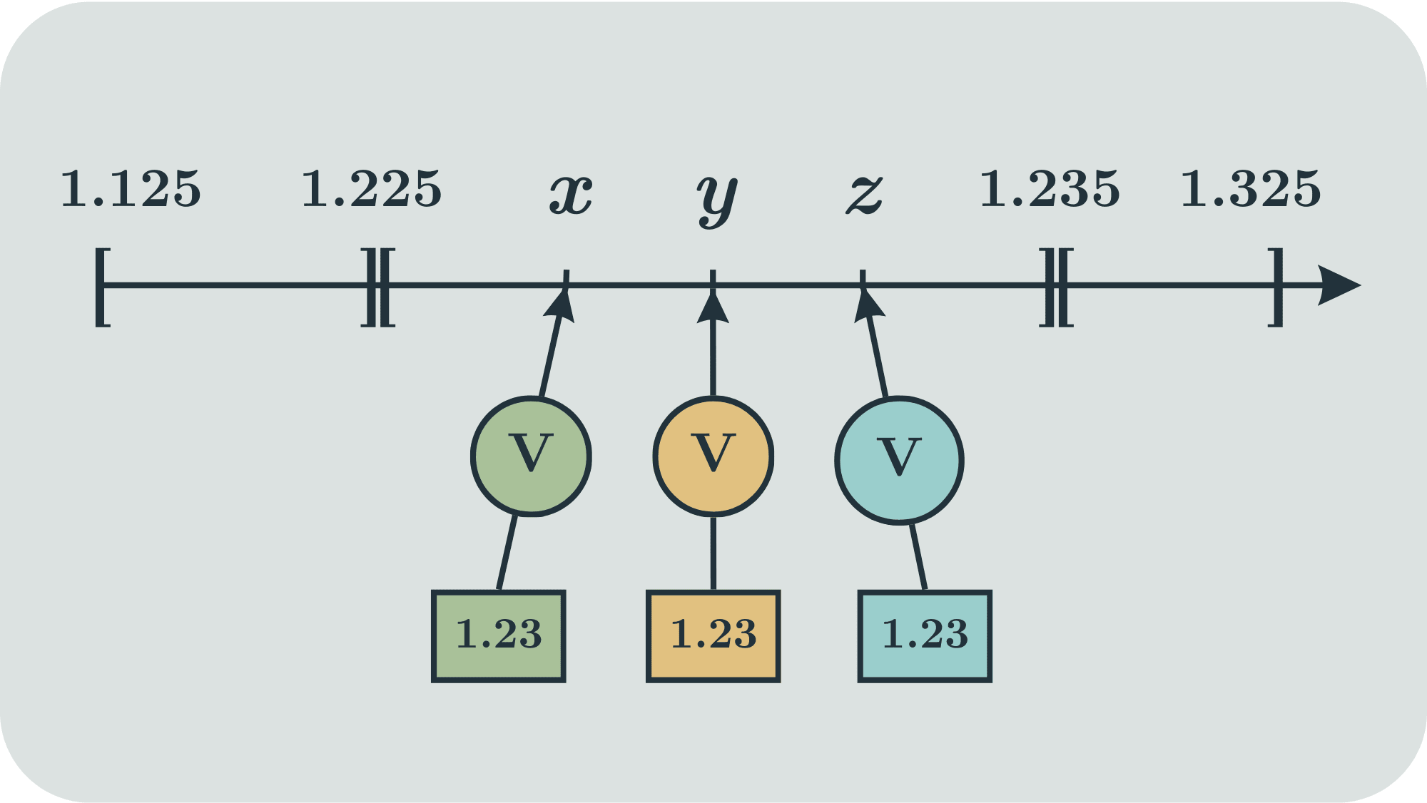
“Consider an ideal voltmeter that is perfectly accurate, but only reads out to a precision of $0.01V$. If a voltage may be any real number, and if, say, a reading of $1.23$ volts means that the measured voltage v satisfies $1.225V\le v\le 1.235V$, then the voltmeter determines a partition of the real line into intervals of length $0.01$. What is ‘known’ about any measured voltage is just that it lies within the cell corresponding to the reading.” 

In other words, any measured number inside the interval $[1.225,1.235]$ provides the same information.

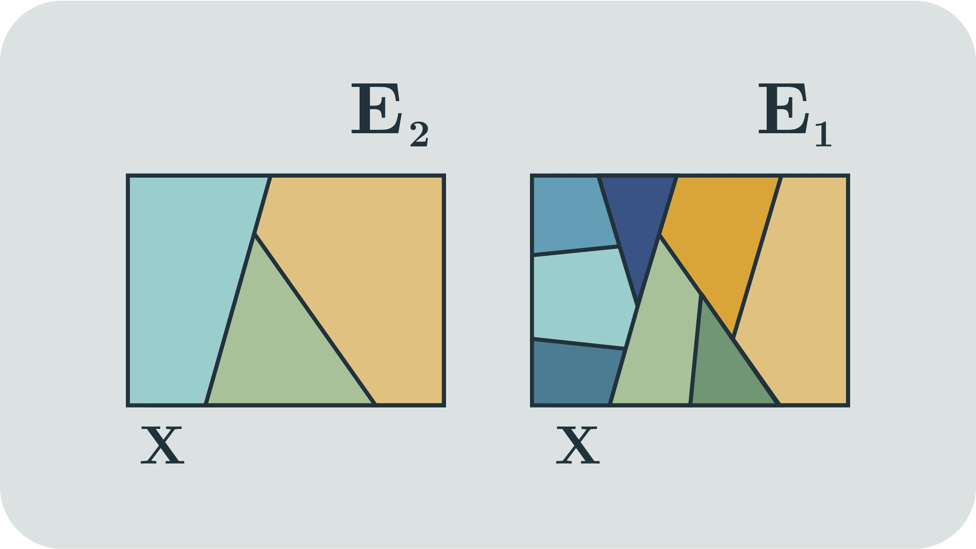
We can also interpret that if $E_1$ and $E_2$ are equivalence relations and $E_1\le E_2$, $E_1$provides us with more information than $E_2$. Thinking of $E_1$ as a partition of a closed region of a plane, it has more cells than $E_2$. The figure below illustrate $E_1$ and $E_2$ as partitions:

On this basis, the finest partition possible for any given set $X$ is

$$P=\left\{\right\{x\};x\in X\}$$

In words, the finest partition is the one in which each $x$ is alone in a cell.

And the equivalence relation associated with $P$ is ^[3]

$$\perp :=\left\{\right(x,x)\in X\times X:x\in X\}$$

Let’s consider, then, our mapping $\gamma$ provides us with the finest equivalence relation possible, that is, 

$$\ker \gamma =\perp$$

Thus, for any $x\in X$, there’s no other $y\in X$ such that $\gamma \left(x\right)=\gamma \left(y\right)$, for, if this wasn’t the case, then $(x,y)\in \ker \gamma$, which is a contradiction because $\ker \gamma =\perp$

Hence, if we assume $\ker \gamma =\perp$, we get that $\gamma$ must be a bijection, and examples such as the one we used above don’t satisfy this new hypothesis. We know that, by our theorem, ${\alpha }_C\circ \gamma =\gamma \circ \alpha$ and $\gamma$ is bijective. This is saying, by definition, that ${\alpha }_C$ and $\alpha$ are isomorphic dynamic systems.

One way to think about isomorphism is that two objects are isomorphic if they’re the same thing with different labels. Thus, with the new assumption, ${\alpha }_C$ not only models $\alpha$ in a weak manner, but faithfully simulates $\alpha$

Note that the key property that ensures faithful simulation here is $\gamma$ injection. If $\gamma$ was only injective, this would also have prevented our pathological example and would also give us an intuition of faithful simulation: we would only need to restrict the co-domain of functions to get a bijection.

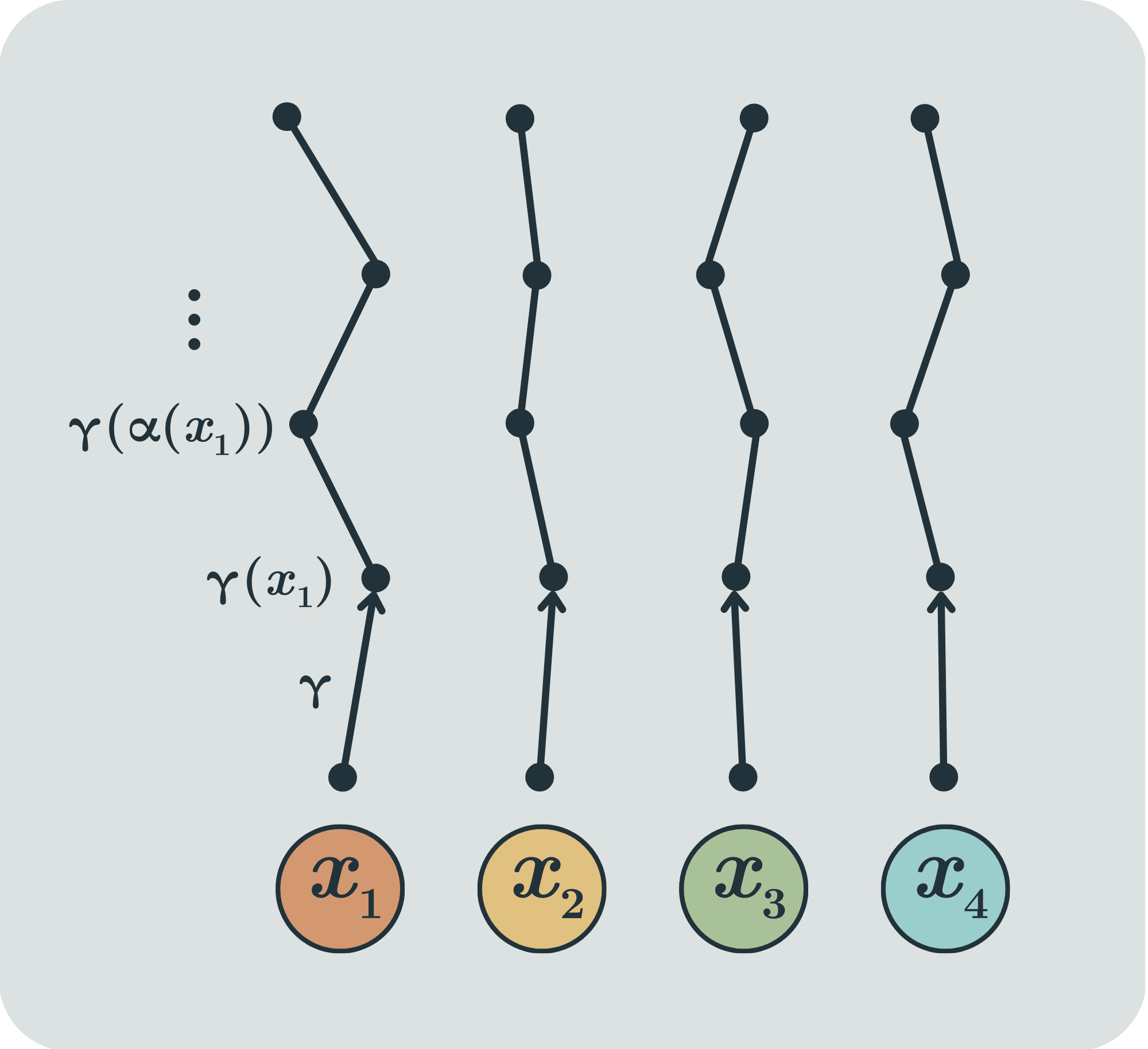
Observability Condition

Now, we’ll consider a slightly more general assumption that can also provide us with a similar result but that we can use to generalize to other setups later.

All the information the FAI can ever get from the ASI starting in a point $x\in X$ is

$$\gamma \left(x\right),\gamma \left(\alpha \right(x\left)\right),\gamma \left(\alpha \right(\alpha \left(x\right)\left)\right),\dots$$

We call $x,\alpha \left(x\right),\alpha \left(\alpha \right(x\left)\right),\dots$ a trajectory and $\gamma \left(x\right),\gamma \left(\alpha \right(x\left)\right),\gamma \left(\alpha \right(\alpha \left(x\right)),\dots$ a trajectory of observations.

Instead of asking $\ker \gamma =\perp$, we ask

$$I:=\bigcap _{n\ge 0}\ker (\gamma \circ {\alpha }^n)=\perp$$

Where ${\alpha }^n={\alpha }^{n-1}\circ \alpha$. We call this the observability condition.

Recall from our algebraic remark that 

$$\bigcap _{n\ge 0}\ker (\gamma \circ {\alpha }^n)=inf\{\ker \gamma \circ {\alpha }^n;n=0,1,2,\dots \}\in E\left(X\right)$$

So our assumption makes sense (i.e, $I$ is indeed an equivalence relation so we can ask it to be equal to $\perp$)

Also note that

$$\bigcap _{n\ge 0}\ker (\gamma \circ {\alpha }^n)=\left\{\right(x,y)\in X\times X;\gamma ({\alpha }^n\left(x\right))=\gamma ({\alpha }^n\left(y\right)),\forall n=0,1,2,\dots \}$$

Hence, if $(x,y)\in I$, the trajectory of observations of $x$ and $y$ is the same.

On the other hand, if $(x,y)\notin I$, then $\gamma \left({\alpha }^{n_0}\right(x\left)\right)\ne \gamma \left({\alpha }^{n_0}\right(y\left)\right)$, for some $n_0=0,1,2,\dots$ - that is, their trajectory of observations is different at least in one point.

Thus, we can think what $I$ is doing is aggregating points $x\in X$ that generate the same observation trajectories into cells $\left[x\right]\in E\left(X\right)$

Asking that $I=\perp$ is to say that each cell $\left[x\right]$ consists of a single point $x$ - that is, the only point that can generate a trajectory of observations $\gamma \left(x\right),\gamma \left(\alpha \right(x\left)\right),\dots \text{is}x\in X$. In other words, given two points $x$ and $y$, their trajectory of observations is different in at least in one step.

We can also interpret this condition in terms of precision: 

• Consider the real line $R$. A partition splits the line into sets (possibly with a single point). Consider a specific partition only made up of intervals. Think of this partition as associated to a weird non-uniform rule with some precision. If the partition intervals have the same length, it's a regular uniform, i.e, equally spaced (but infinitely wide) rule. The rule measures whether two points are in the same cell of the partition or not.
• Suppose we move around all the points according to $\gamma$ in the first time-step, then to $\gamma \circ \alpha$ in the second and so on.
• Each update of the points is associated with a different partition. Taking the intersection of the partitions up to a finite time-step updates our rule with more precision, because the intersection of partitions is always a finer partition.
• In the limit, the partition is $I$, and saying $I=\perp$ is saying that the rule of this partition (updated after all time-steps) can distinguish between any point. We say this rule has infinite precision.

Thus, the observability condition ensures that the information the FAI receives has infinite precision.

Obs.: Note that this condition of “infinite precision” is different from another condition that we call “perfect information”:

• "Infinite precision" states that the FAI can always tell apart two given trajectories of observations.
• "Perfect information" states that given a signal the FAI receives, it's possible to perfectly reconstruct the ASI state that generated that signal.

Let the initial ASI states be $x\in X$, then $\alpha \left(x\right)$, then ${\alpha }^2\left(x\right)$and so on. Comparing the two assumptions:

• $\ker \gamma =\perp$ implies that $x$ is uniquely determined to the FAI - FAI observes $\gamma \left(x\right)$and since $\ker \gamma =\perp$ implies $\gamma$ injective, $x$ is the only ASI state that can yield this observation $\gamma \left(x\right)$. In other words, observation from the first time-step implies $x$ is uniquely determined to the FAI 
• $I={\bigcap }_{n\ge 0}\ker (\gamma \circ {\alpha }^n)=\perp$ implies, by considerations above, that after long enough time-steps, $x$ is uniquely determined to the FAI
• Mathematically, it’s clear that $\ker \gamma =\perp$ implies $I=\perp$ (because I is the infimum of a set and $\ker \gamma$ belongs to this set, thus $I\le \perp )$

Hence, it’s reasonable to think of the observability condition as a generalization of $\ker \gamma =\perp$, both in terms of information structure intuition and mathematically.

Example 2 - Dyadic transformation

• Suppose we're looking at numbers between 0 and 1 in decimal notation. So any number is of the form $x=0.a_1{a}_2\dots a_n\dots$, where each $a_i$ is a binary digit, i.e, $a_i=0$ or $a_i=1$.
• Let the dynamics be $\alpha \left(x\right)$= $2x\mathrm{mod}1$
• Now, when we double a binary digit, we're only shifting the digits one place to the left (so $2x=a_1.a_2{a}_3\dots a_n\dots$) and $2x\mathrm{mod}1=0.a_2{a}_3\dots a_n\dots$ (because if $a_1=1$, the $\mathrm{mod}1$ gets rid of $a_1$ and so $2x\mathrm{mod}1$ = $0.a_2{a}_3\dots a_n\dots$ , and if $a_1=0$, the $\mathrm{mod}1$ does nothing. Then, the dynamics of the system just shifts every bit to the right and replaces the most significant digit (before the period) with 0
• Hence, $\alpha \left(x\right)=0.a_2{a}_3\dots a_n\dots$;  ${\alpha }^2\left(x\right):=\alpha \circ \alpha \left(x\right)=0.a_3{a}_4\dots a_n\dots$ and so on...
• Suppose $\gamma (0.a_1{a}_2\dots a_n\dots )=a_1$ for all numbers in this form. This means that the only information we have available is the first digit after the period.
• Now suppose we have a system that starts in $x\left(0\right)=x_0$ and evolves according to $\alpha .$Then, $x(t+1)=\alpha \left(x\right(t\left)\right)$ and $\gamma$ is capable of uniquely determining $x_0$. Indeed, $\gamma \left(x\right)=a_1,\gamma \left(\alpha \right(x\left)\right)=a_2,\gamma \left({\alpha }^2\right(x\left)\right)=a_3,\dots ,\gamma \left({\alpha }^n\right(x\left)\right)=a_{n+1},\dots$

Note that in this scenario, $\gamma$ is able to determine every digit of $x_0$, which has an infinite amount of digits. This illustrates well why observability relates to infinite precision.

Lemma: Generalized Feedback Condition

Before we check that the observability condition yields an analogous result to $\ker \gamma =\perp$, we need to construct a lemma.

Recall that the feedback condition states that $\ker \gamma \le \ker \gamma \circ \alpha$. This, in turn, implies that 

$$\ker \gamma \le \ker \gamma \circ \alpha \le \ker \gamma \circ {\alpha }^2\le \ker \gamma \circ {\alpha }^3\le \dots \le \ker \gamma \circ {\alpha }^k\le \dots$$

Note that in the proof^[4], it is important to use $s,t\in X$. In the next post, we’ll consider a larger set and one crux of the argument will be to ask that $s$ and $t$ remain in a given set.

The theorem

We can now derive a more specific version of the theorem by assuming the feedback condition and the observability condition.

We’ll see that, in our setup, observability and feedback trivially implies $\gamma$ bijection, but this will not be necessarily true in a more general setup, and we will use the same idea of proof to extend this to the more general scenario.

By the generalized feedback condition, 

$$\ker \gamma \le \ker \gamma \circ \alpha \le \ker \gamma \circ {\alpha }^2\le \ker \gamma \circ {\alpha }^3\le \dots \le \ker \gamma \circ {\alpha }^k\le \dots$$

Which implies

$$inf\{\ker \gamma \circ {\alpha }^n;n=0,1,2,\dots \}=\ker \gamma$$

(Because the infimum is the greatest lower bound)

By observability, 

$$inf\{\ker \gamma \circ {\alpha }^n;n=0,1,2,\dots \}=\perp$$

Thus, we derive that $\ker \gamma =\perp$, the initial condition we used to show that $\gamma$ is bijective.

Obs.: The general mathematical relation between the assumptions we discussed in our setup is as follows: 

• $\ker \gamma =\perp ⟹$observability
• observability and feedback $⟹\ker \gamma =\perp$
• Note that $\ker \gamma =\perp$$⟺$$\gamma$ bijection, hence
  • $\gamma$ bijection$⟺$observability and feedback

To finish up the discussion, let’s restate mathematically the complete theorem with all the assumptions and interpret it.

Theorem: Internal Model Principle simplified

Let $\alpha :X\to X$ and $\gamma :X\to X_C$ surjective.

• (The FAI necessarily models the ASI) If $\ker \gamma \le \ker \gamma \circ \alpha$ (feedback), then
  • ${\alpha }_C:X_C\to X_C$ is the unique map determined by ${\alpha }_C\circ \gamma =\gamma \circ \alpha$
• (The model is faithful) Additionally, if $inf\{\ker \gamma \circ {\alpha }^n;n=0,1,2,\dots \}=\perp$ (observability), then
  • $\gamma :X\to X_C\text{bijection}$

Thus, $\alpha$ and ${\alpha }_C$ are isomorphic.

If $\alpha :X\to X$ represents the ASI dynamics and $\gamma :X\to X_C$ represents the information map from the ASI to the FAI, then

• If the FAI is an autonomous dynamic system, there’s a unique map defined on FAI states that could possibly model the ASI.
• If, additionally, the FAI can distinguish between the ASI’s different trajectories, then this unique map faithfully represents the ASI, in the sense that they’re isomorphic.

The need to generalize

Clearly, this doesn’t accurately represent a real world scenario of scalable oversight and is also a very specific theorem with strong assumptions that a lot of real systems don't satisfy:

1. We’re assuming the ASI dynamics to be discrete and deterministic
   1. The discrete assumption seems more or less acceptable, given that
      1. Real world computers are finite and discrete
      2. Even for continuous or mixed phenomena, good discretized models can provide us a lot of insight
   2. The deterministic assumption feels more complex to handle and depends on the nature of the ASI - would the ASI be just a super big calculator with fixed weights? Would it take action under uncertainty?
2. As the theorem is now, it can’t represent any example of an observation map that is not a bijection (since feedback and observability together are equivalent to $\gamma$ bijection). This is a problem because
   1. The observation map being a bijection means that the information the FAI receives from the ASI is perfect: we can uniquely reconstruct the ASI sequence of states via the FAI sequence of observations (i.e, ${\gamma }^{-1}$ is well-defined and unique). This is quite a strong assumption.
   2. It seems it would be more interesting and general if the theorem applied to systems without perfect information; that is, if the theorem guaranteed that even systems with less than perfect information could develop a faithful internal model.
   3. This implies that $X$ and $X_C$ have the same cardinality.
      1. Would a weaker and stronger model have the same cardinality? Intuitively, we would expect the cardinality of the ASI stateset to be greater than FAI stateset.

Nonetheless, this theorem can be a (simplistic) starting point to think about formalizing AI control questions. It may also help answer alignment-relevant questions such as the agent-structure problem, as we'll see in the second post.

We can solve part of the problem by relaxing a few assumptions we made:

• We allowed the FAI to be autonomous whenever the ASI is in any state (feedback states that $\ker \gamma \le \ker \gamma \circ \alpha$). We could have considered that there’s a set $K\subseteq X$ of ASI states where the FAI is allowed to be autonomous.
• It could be the case that the FAI doesn't receive information directly from the ASI, but instead that the ASI interacts with the world and the FAI receives information from this world.

We'll show a version of the theorem that can be applied in more general setups and that this general version actually solves the problem pointed in 2. (i.e, $\gamma$ bijection) in the second post.

 

 

1. ^{^}

   Supervisory Control of Discrete-Event Systems, (2019) Cai & Wonham as section 1.5

2. ^{^}

   This is called the kernel of a function because it's somewhat analogous to the kernel of a linear map from linear algebra, or the kernel of a homomorphism from abstract algebra. Here, instead of being the set of all things that get sent to zero, we're partitioning the whole domain into sets of things that get sent to the same value of the codomain

3. ^{^}

   The symbol $\perp$ is read as "bottom". We use this name and symbol because the equivalence relation $\perp$ is smaller than any other in our (partial) ordering defined on the set of equivalence relations over $X$

4. ^{^}

   We can prove this fact by a simple induction on $k$, but we’ll outline the proof for didactic purposes (it will help readers understand why, when extending the theorem, we need to ask for some set to be $\alpha$-invariant): 

   • Base case: $k=1$ is the feedback condition, which we assume to be true
   • Induction hypothesis: Suppose all the inequalities hold for $k>2$, that is, 

   $$\ker \gamma \le \ker \gamma \circ \alpha \le \ker \gamma \circ {\alpha }^2\le \ker \gamma \circ {\alpha }^3\le \dots \le \ker \gamma \circ {\alpha }^k$$

   • Inductive step: Now, we must prove 

   $$\ker \gamma \le \ker \gamma \circ \alpha \le \ker \gamma \circ {\alpha }^2\le \ker \gamma \circ {\alpha }^3\le \dots \le \ker \gamma \circ {\alpha }^k\le \ker \gamma \circ {\alpha }^{k+1}$$

   • By induction hypothesis, $(x,y)\in \ker \gamma ⟹\left(\gamma \right({\alpha }^k\left(x\right)),\gamma ({\alpha }^k\left(y\right)\left)\right)\in \ker \gamma$. Let ${\alpha }^k\left(x\right)=s$ and ${\alpha }^k\left(y\right)=t$. Since $\alpha :X\to X$, we know $s,t\in X$ and by above we know $(s,t)\in \ker \gamma$. By Feedback, $(s,t)\in \ker \gamma ⟹\left(\alpha \right(s),\alpha (t\left)\right)\in \ker \gamma$. Thus,  $\left({\alpha }^{k+1}\right(x),{\alpha }^{k+1}(y\left)\right)=\left(\alpha \right({\alpha }^k\left(x\right)),\alpha ({\alpha }^k\left(y\right))=(\alpha \left(s\right),\alpha \left(t\right))\in \ker \gamma$
   • The rest of the inequalities follow by transitivity
   • Hence, the proof follows by induction

0 comments

Comments sorted by top scores.