Individual Utilities Shift Continuously as Geometric Weights Shift

post by StrivingForLegibility · 2024-08-07T01:41:10.071Z · LW · GW · 0 comments

Contents

  High Level Overview
  Parameterizing the Pareto Hypersurface
  Computing the Harsanyi Weights
  The Harsanyi Bundle
  The Harsanyi Shadow
    The Harsanyi Shadow of Convex Hulls
    The Harsanyi Shadow of a Hyperplane
    The Harsanyi Shadow of a Corner
    The Harsanyi Shadow of Curved Hypersurfaces
  Inverting the Hadamard Product
  Normalizing the Harsanyi Shadow
    Normalizing the Interior of the Harsanyi Shadow is Injective
    Normalizing the Harsanyi Shadow is Surjective
  Moving Continuously Across the Harsanyi Bundle
    The Challenge of Continuity Around the Boundary
    Motivating Example
    How to Achieve Continuity Anyway
None
No comments

This is a supplemental post to Geometric Utilitarianism (And Why It Matters) [LW · GW], in which I show that when all agents have positive weight ${\psi }_i$, the optimal geometric weighted average moves continuously across the Pareto frontier as we change those weights. I also show that we can extend this continuity result to all weights $\psi$, if we're willing to accept an arbitrarily good approximation of maximizing $G(\_,\psi )$. I think of this as a bonus result which makes the geometric average a bit more appealing as a way to aggregate utilities, and the main post [LW · GW] goes into more detail about the problem and why it's interesting.

High Level Overview

How does changing $\psi$ affect the optima of $G(\_,\psi )$? Ideally, we'd like a small change in the weights assigned to each agent to cause a small change in the resulting joint utility $p$. In other words, we would like $p\left(\psi \right)=\underset{u\in F}{\arg max}G(u,\psi )$ to be continuous. It turns out this is true when ${\psi }_i>0$ for all agents, and there's at least one way to create a continuous function $\psi \to p$ that works for all $\psi \in {\Delta }^n$ and is an arbitrarily good approximation of $G(\_,\psi )$ maximization.

We've already solved [LW · GW] the inverse problem: given a point $p$ and Harsanyi weights $\varphi$ which make $p$ optimal according to $H(\_,\varphi )$, find geometric weights $\psi$ that make $p$ optimal according to $G(\_,\psi )$.

$\psi =\frac{p\odot \varphi }{p\cdot \varphi }$

So we already have $\psi (p,\varphi )$, which is a smooth function of its inputs where it's defined.^[1] 

It turns out we can invert this function and recover $(p,\varphi )$ from $\psi$ when $p_i>0$ and ${\varphi }_i>0$ for all agents. This is the interior of what we'll be calling the Harsanyi Bundle; the set of all of the pairs $(p,\varphi )$ which are consistent with our Pareto frontier $P$. This post will show that there is a bijection between the interior of the Harsanyi Bundle and the interior of the set of all valid weights ${\Delta }^n$.

So we have a smooth bijection $(p,\varphi )\to \psi$ between these two subsets of $R^{2n}$ and $R^n$ respectively. And thankfully we're doing calculus, where this is sufficient to establish that the inverse function $\psi \to (p,\varphi )$ is at least continuous.^[2] And that is the main result this post sets out to prove: that individual utilities shift continuously as geometric weights shift.

Establishing this homeomorphism with the interior of ${\Delta }^n$ means that the interior of the Harsanyi Bundle is an $n-1$ dimensional manifold. The last part of this post involves extending our map $\psi \to (p,\varphi )$ so that it's continuous across all of ${\Delta }^n$. My current favorite way to do this is to introduce a new continuous function $\beta \left(\psi \right)$ which maps all weights $\psi$ into the interior of ${\Delta }^n$, and then using those positive weights to find the unique optimum of $G(\_,\beta (\psi \left)\right)$.

Parameterizing the Pareto Hypersurface

Just like the Harsanyi hyperplane $H$, we can think of the Pareto frontier $P$ as a set of joint utilities, or as a function $P:R^{n-1}\to R^n$ which maps utilities for the first $n-1$ agents into that set. $P_n\left(v\right)$ returns the highest feasible utility agent $n$ can receive, given that the first $n-1$ agents receive utilities defined by $v$. (Or undefined if $v$ is already infeasible.) And $P_i\left(v\right)=v_i$ for $i<n$.

We can think of $P$ as a hypersurface that lies "above" the feasible utilities for the first $n-1$ agents.

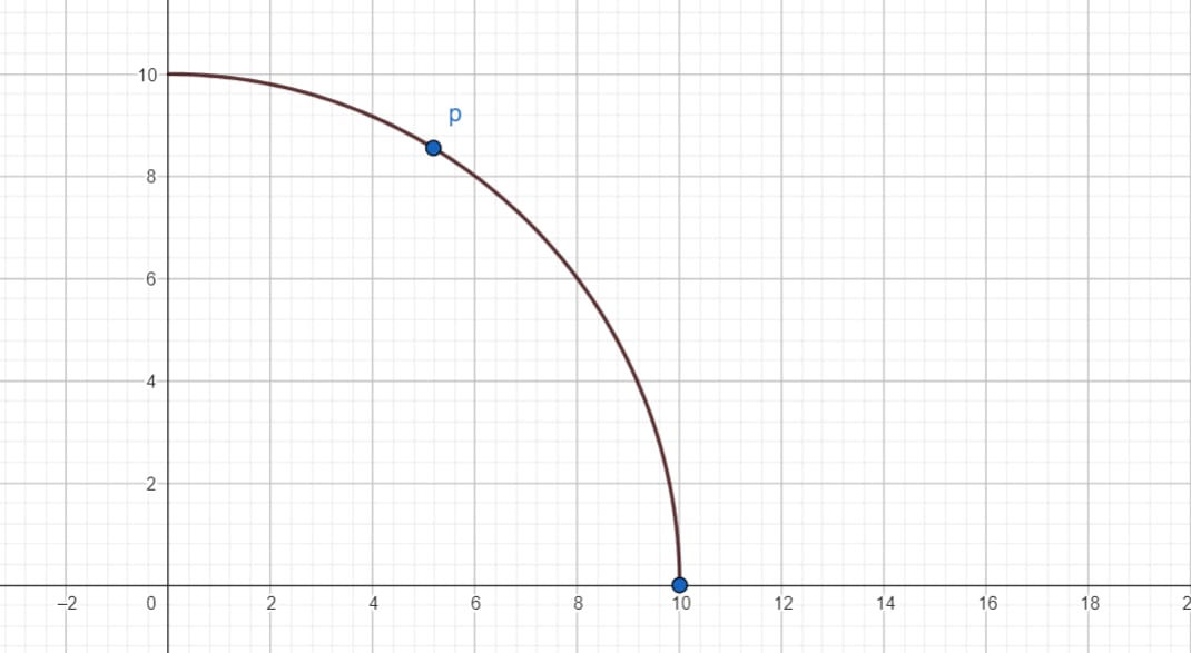
Where $P$ is differentiable, the Harsanyi hyperplane $H$ for a point $p$ lines up exactly with the tangent hyperplane at that point $T_{p}P$.^[3] The Harsanyi weights $\varphi$ are orthogonal to $T_{p}P$, and so there is only one choice of $\varphi$ which causes $p$ to maximize $H(\_,\varphi )$.

But where $P$ isn't differentiable, such as at corners, the tangent hyperplane isn't defined, and there can be multiple hyperplanes $H$ which keep $F$ all on one side. And so there can be many consistent values for $\varphi$ at these points.

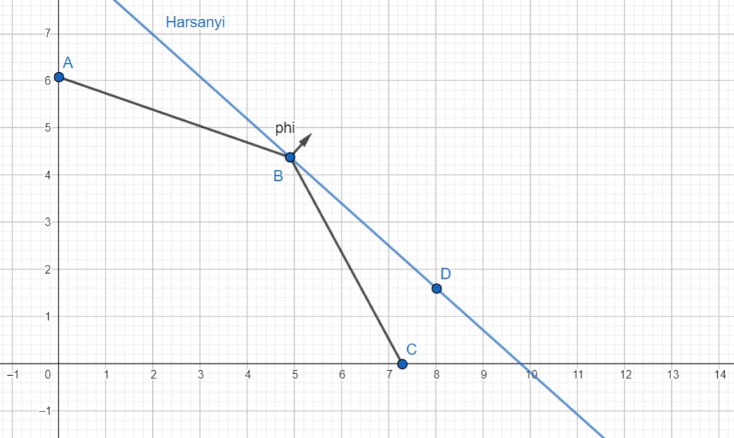
When the slope of $P$ jumps discontinuously at a point $p$, these slopes and all of the slopes in between can be used to find all of the valid assignments for $\varphi$ at $p$. When $F$ looks like a jewel with multiple flat faces meeting at corners, we can identify $\varphi \left(F_i\right)$ for each face $F_i$. The valid assignments for $\varphi$ at a corner $p$ are all of the convex combinations of $\varphi \left(F_i\right)$ for all of the faces $F_i$ that meet at that corner $p$.^[4] $\varphi$ only acts like a function when there is only one valid assignment, and in general we can call the set of all valid assignments $\Phi \left(p\right)$.

Computing the Harsanyi Weights

So far we've been treating $\varphi$ as coming from a black box, but now that we've parameterized $P$ it's actually straightforward to compute $\varphi$ at differentiable points $p\in P$. 

What we have is a function $P:R^{n-1}\to R^n$, and what we want to do is construct a new function $\hat{P}:R^n\to R$ such that $P$ is a level set of $\hat{P}$. This causes the gradient $\nabla \hat{P}$ to be orthogonal to $P$, which is exactly the direction we want $\varphi$ to point!

Starting from $u_n=P_n\left(v\right)$, we can rearrange this to get $0=P_n\left(v\right)-u_n$. Which is a level set of $\hat{P}\left(u\right)=P_n\left(v\right(u\left)\right)-u_n$. 

• $\frac{\partial \hat{P}}{\partial u_i}=\frac{\partial P_n}{\partial v_i}$ for $i<n$
• $\frac{\partial \hat{P}}{\partial u_n}=-1$

And that's $\nabla \hat{P}$! To get $\varphi$, all we have to do is normalize $\nabla \hat{P}$ so that its components sum to 1. If we use $\overrightarrow{1}\in R^n$ to denote the vector whose components are all 1, then

$\varphi =\frac{\nabla \hat{P}}{{\sum }_{i=1}^n\nabla {\hat{P}}_i}=\frac{\nabla \hat{P}}{\nabla \hat{P}\cdot \overrightarrow{1}}$

For an arbitrary surface that might wiggle up and down, this procedure won't necessarily guarantee that $\varphi \in {\Delta }^n$. But this is a Pareto frontier, where we know that $\frac{\partial P_n}{\partial v_i}\le 0$; increasing agent $i$'s utility never increases the feasible utility for agent $n$. $P$ might wiggle down, but it never wiggles up, and that keeps $\varphi$ in its valid range wherever $P$ is differentiable.

We also know that increasing $p_i$ never decreases ${\varphi }_i$. So $\frac{\partial {\varphi }_i}{\partial p_i}\ge 0$, which implies that $\frac{{\partial }^2{P}_n}{\partial v_i^2}\le 0$. We'll use this fact later when looking at curves which increase $p_i$, and thus monotonically increase ${\varphi }_i$.

The Harsanyi Bundle

In order to claim that $\psi (p,\varphi )$ changes continuously as we change $p$ and $\varphi$, we need to be able to define what that even means in the context of $P$. If we take a curve $\gamma :R\to P$ that travels continuously along $P$, then $\varphi \left(\gamma \right)$ will change discontinuously at corners no matter how we break ties.

All pairs $(p,\varphi )$ come from $P\times {\Delta }^n$, but let's restrict our attention to a subset I'll denote $(P,\Phi )$ which contains all of the valid pairs $(p,\varphi )$ which are consistent with $P$. So $(P,\Phi )=\left\{\right(p,\varphi )|p\in P,\varphi \in \Phi (p\left)\right\}$. It turns out this forms a surface in $2n$-dimensional space I'll call the Harsanyi Bundle, analogous to the tangent bundle in differential geometry.^[5]

Where $P$ is differentiable, there is only one valid assignment for $\varphi$. So any continuous curve $\gamma$ through these parts of $P$ corresponds to a continuous curve $\chi$ through $(P,\Phi )$. At non-differentiable points $p$, $\chi$ can travel continuously to any point in $(p,\Phi (p\left)\right)$, including the endpoints which allow it to continue on to other parts of the Harsanyi bundle.

When projected onto $P$, $\chi$ looks like a continuous curve along $P$ that sometimes hangs out at corners while $\varphi$ rotates to line up with the next face along the path of $\chi$.

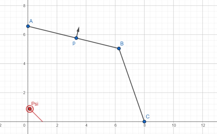
The upshot is that any two points in $(P,\Phi )$ can be reached using continuous paths, so we can think of it as a single continuous surface embedded in $2n$-dimensional space. And these correspond to continuous changes in geometric weight $\psi$.

The Harsanyi Shadow

We're trying to invert $\psi :(P,\Phi )\to {\Delta }^n$, which has the formula

$\psi =\frac{p\odot \varphi }{p\cdot \varphi }$

If we were writing a program to compute $\psi (p,\varphi )$, our first step would be to compute $p\odot \varphi$. This is the element-wise product of $p$ and $\varphi$, also called their Hadamard product. We can think of $\odot$ as a linear map $\odot :R^n\times R^n\to R^n$, which takes us from $2n$-dimensional space back down to $n$-dimensional space. And it turns out that the image $\odot (P,\Phi )$, consisting of all the points $p\odot \varphi$ where $(p,\varphi )\in (P,\Phi )$, forms a hypersurface that lies "under" $P$.

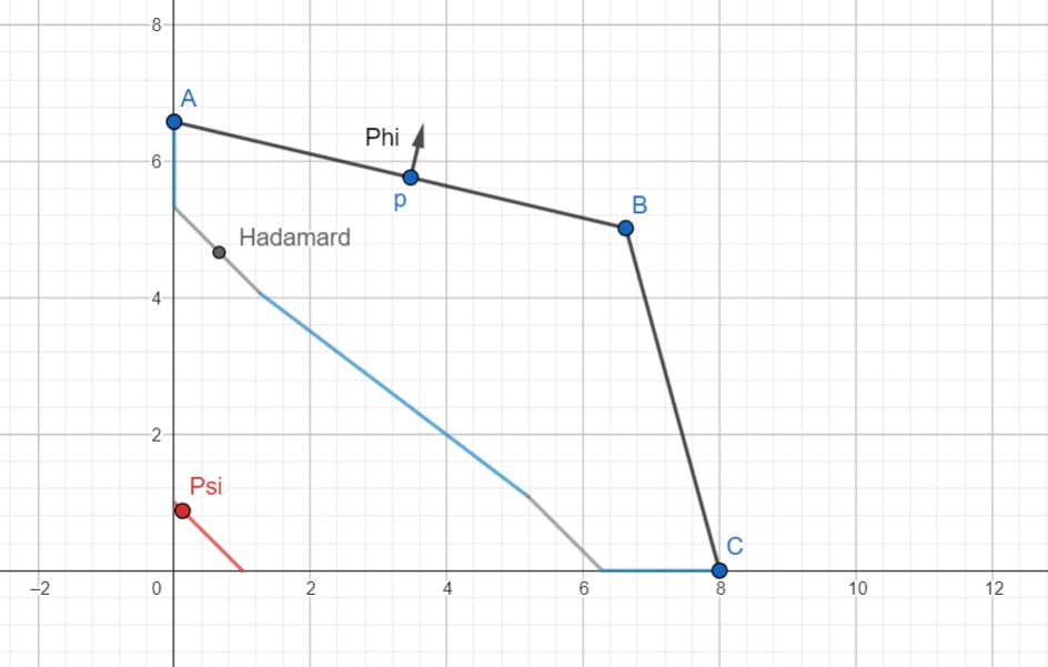
I'm calling this hypersurface the Harsanyi Shadow of $P$, and I think of it as a projection of the Harsanyi Bundle back down into $n$-dimensional space. As always if there's a standard name or notation for something I generally prefer to switch to that. We'll also show that at least the interior of the Harsanyi Shadow is an $n-1$ dimensional manifold, since it's in smooth bijection with the interior of ${\Delta }^n$.

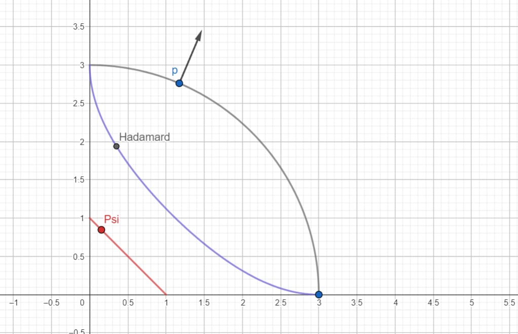
In this example, the grey line segments on the Harsanyi Shadow correspond to black line segments $\overline{AB}$ and $\overline{BC}$ on the Pareto frontier. The blue line segments correspond to the points $A$, $B$, and $C$, and the values of $\varphi$ which make them optimal according to $H(\_,\varphi )$.

In particular, points like A and C on the boundary of $P$, and thus on the boundary of $(P,\Phi )$, correspond to "wings" on the Harsanyi Shadow which lie on the same line from the origin. When these wings are normalized onto ${\Delta }^n$ in the next step of calculating $\psi$, these will all end up at the same point. 

The Harsanyi Shadow of Convex Hulls

Any convex set like $F$ can be thought of as the convex hull of a set of points $X$. When $X$ is finite, which is generally the case when it represents something like a deterministic policy for each agent, $P$ will be made up of flat surfaces that meet at corners. These correspond to two types of surface in $(P,\Phi )$:

• "Horizontal" surfaces where $\varphi$ is constant and $p$ is changing
• "Vertical" surfaces where $p$ is constant and $\varphi$ is changing.

When one element of a Hadamard product is constant, such as $\varphi$ for "horizontal" surfaces, we can think of it as a linear map $\odot (\_,\varphi ):R^n\to R^n$. This corresponds to a diagonal matrix, which we can write in diagonal notation $diag\left(\varphi \right)$ or in components as $\odot (\_,\varphi {)}_{ij}={\delta }_{ij}{\varphi }_i$. This is invertible if and only if ${\varphi }_j>0$ for all agents. So flat surfaces on $P$ map linearly to flat surfaces on $(P,\Phi )$, which map linearly to flat surfaces on $\odot (P,\Phi )$. $\odot (\_,\varphi (H\left)\right):H\to R^n$ acts linearly when restricted to points on the same hyperplane $H$.

Since we have an explicit formula for $\varphi$, we can use that to write down an explicit formula for $p\odot \varphi$

$p\odot \varphi =p\odot \frac{\nabla \hat{P}}{\nabla \hat{P}\cdot \overrightarrow{1}}=\frac{1}{\nabla \hat{P}\cdot \overrightarrow{1}}(p\odot \nabla \hat{P})$

In components, this looks like 

• $(p\odot \varphi {)}_i=\frac{p_i}{\nabla \hat{P}\cdot \overrightarrow{1}}\frac{\partial P_n}{\partial v_i}$ for $i<n$
• $(p\odot \varphi {)}_n=-\frac{p_n}{\nabla {\hat{P}}_i\cdot \overrightarrow{1}}$

The Harsanyi Shadow of a Hyperplane

We can approximate any Pareto frontier using pieces of hyperplanes, and the Harsanyi Shadow of this approximation will be made up of the pieces of $H\odot \varphi \left(H\right)$. And it turns out that these pieces are all parallel to ${\Delta }^n$! Which helps a lot in understanding the geometry of the Harsanyi Shadow, and why the interior pieces are in one-to-one correspondence with pieces of ${\Delta }^n$.

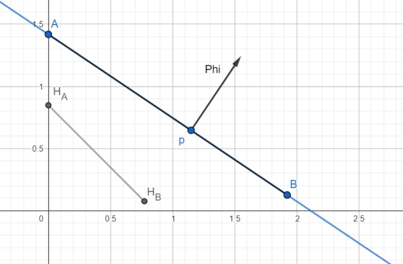
I noticed this playing around with examples, and I recommend playing with this one. If you pick two points A and B, you can draw the line between them, and calculate $\varphi$ for that line. $\odot (\_,\varphi )$ is always a linear map, and when ${\varphi }_i>0$ for all agents, it's an invertible linear map that maps this line to another line on the Harsanyi Shadow. And it turns out this line on the Harsanyi Shadow will always have slope $-1$! Just like the standard $2$-simplex ${\Delta }^2$ where $\varphi$ and $\psi$ live. And in general, $H\odot \varphi \left(H\right)$ is a hyperplane with the same slope as ${\Delta }^n$, as long as ${\varphi }_i>0$ for all agents.

This is why the grey line segments in our example were parallel to the red line segment of valid weights; flat surfaces on the Pareto frontier map onto flat surfaces on the Harsanyi Shadow that are parallel to ${\Delta }^n$.

To see why this happens for hyperplanes in general, we can use the fact that $\varphi$ is orthogonal to $H$ at $p$ to write down the normal equation for $H$. It's all of the points $u\in R^n$ which satisfy

$\varphi \cdot (u-p)=0$

The image of $H$ after going through the map $\odot (\_,\varphi )$, which we can denote $H\odot \varphi$ is all of the points $u\odot \varphi$ where $u\in H$. One such point is $p\odot \varphi$, and in general there will be a vector I'll suggestively call $\delta \in R^n$ which is orthogonal to $H\odot \varphi$. This normal vector $\delta$ satisfies the equation

$\delta \cdot (u\odot \varphi -p\odot \varphi )=0$

Since the Hadamard product is distributive and commutative, we know that

$u\odot \varphi -p\odot \varphi =\varphi \odot (u-p)$

Which means we can rewrite the normal equation for $H\odot \varphi$ as

$\delta \cdot (\varphi \odot (u-p\left)\right)=0$

Here I needed to go back to component notation to know how I could simplify that equation further.

${\sum }_{i=1}^n{\delta }_i\left({\varphi }_i\right(u_i-p_i\left)\right)=0$

${\sum }_{i=1}^n{\delta }_i{\varphi }_i(u_i-p_i)=0$

$(\delta \odot \varphi )\cdot (u-p)=0$

This is great, because we also know from the normal equation for $H$ that

$\varphi \cdot (u-p)=0$

And in fact, we know that any scalar multiple $\lambda \varphi$ is also orthogonal to $H$

$\lambda \varphi \cdot (u-p)=0$

And so one family of solutions for $\delta$ comes from solving

$\delta \odot \varphi =\lambda \varphi$

Which has the solution ${\delta }_i=\lambda$.

$\delta =\lambda \overrightarrow{1}$

This line is orthogonal to $H\odot \varphi$, and it's also orthogonal to ${\Delta }^n$! So $H\odot \varphi$ and ${\Delta }^n$ are parallel in the sense that they're orthogonal to the same line. And when ${\varphi }_i>0$ for all agents, $H\odot \varphi$ is a hyperplane with the same normal vector as ${\Delta }^n$.

The Harsanyi Shadow of a Corner

At a corner $p$, the Harsanyi Shadow $p\odot \Phi \left(p\right)$ will be a subset of $p\odot {\Delta }^n$. And when $p_i>0$ for all agents, $\odot (p,\_)$ is an invertible linear map that takes the standard simplex ${\Delta }^n$ to a simplex with a similarly-negative slope in all directions.

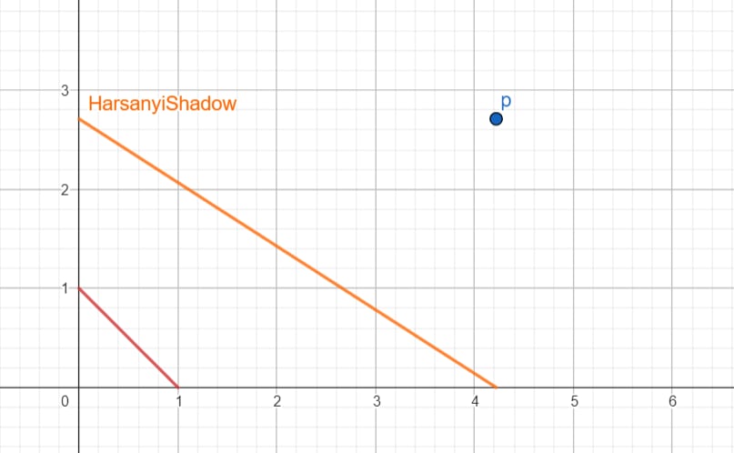
Since $p_i\ge 0$, $\odot (p,\_)$ can't flip the sign of the slope of this simplex. Together with the results from the previous sub-section about hyperplanes, we can conclude that the Harsanyi Shadow of $(P,\Phi )$ never has positive slope. (Just like $P$ and ${\Delta }^n$.) The main relevance for us is that in the interior, the Harsanyi Shadow never slopes up in a way that would allow two points to lie on the same line from the origin, which would violate injectivity when we normalize it onto ${\Delta }^n$. (That line would need to have positive slope, which the Harsanyi Shadow never has.)

The Harsanyi Shadow of Curved Hypersurfaces

Where $P$ curves differentiably, these correspond to "diagonal" surfaces where $p$ and $\varphi$ are both changing.

Inverting the Hadamard Product

When can we invert $\odot$ and recover $(p,\varphi )$ from $p\odot \varphi$? When $p_i>0$ and ${\varphi }_i>0$ for all agents! This leads to ${\psi }_i>0$ for all agents, and we saw here [LW · GW] that this ensures that $G(\_,\psi )$ has a unique optimum among $F$. (And finding this optimum is exactly what we mean by recovering $p$.)

Why is this true? Here's where we use the fact that $\frac{\partial {\varphi }_i}{\partial p_i}\ge 0$, that increasing $p_i$ never decreases ${\varphi }_i$. In order for $\odot$ to cause a collision, there would need to be two points $(p,\varphi ),(q,\tau )\in (P,\Phi )$ such that $p\odot \varphi =q\odot \tau$. This corresponds to $n$ equations that look like

$p_i{\varphi }_i=q_i{\tau }_i$

Holding $p_i{\varphi }_i$ constant, this becomes the equation of a hyperbola. And the claim is that if $p_i>0$ and ${\varphi }_i>0$ for all agents, then these equations only have one solution among $(P,\Phi )$, and it's $(p,\varphi )$.

For concreteness, suppose $p_i=2$ and ${\varphi }_i=3$. Then $p_i{\varphi }_i=6$, and we could try picking $q_i>p_i$, like $q_i=3$. But this would require ${\tau }_i=2$, which can't happen because $\frac{\partial {\varphi }_i}{\partial p_i}\ge 0$; on the Pareto frontier, increasing the utility assigned to an agent can't decrease the Harsanyi weight they must have been assigned. The same problem happens if we try to assign $q_i<p_i$. The only solution is $q_i=p_i$.

So for the interior of the Harsanyi Bundle $(P,\Phi )$, projecting by $\odot$ is injective and we can uniquely recover $(p,\varphi )$ from $p\odot \varphi$. 

Normalizing the Harsanyi Shadow

Once we have $p\odot \varphi$, we can calculate $p\cdot \varphi$ by simply adding up all of its elements! $p\cdot \varphi ={\sum }_{i=1}^n{p}_i{\varphi }_i$. This is a single number, which acts on $p\odot \varphi$ by scaling it down to land on ${\Delta }^n$, the hypersurface of weights that add up to 1. And that's $\psi$!

$\psi =\frac{p\odot \varphi }{p\cdot \varphi }$

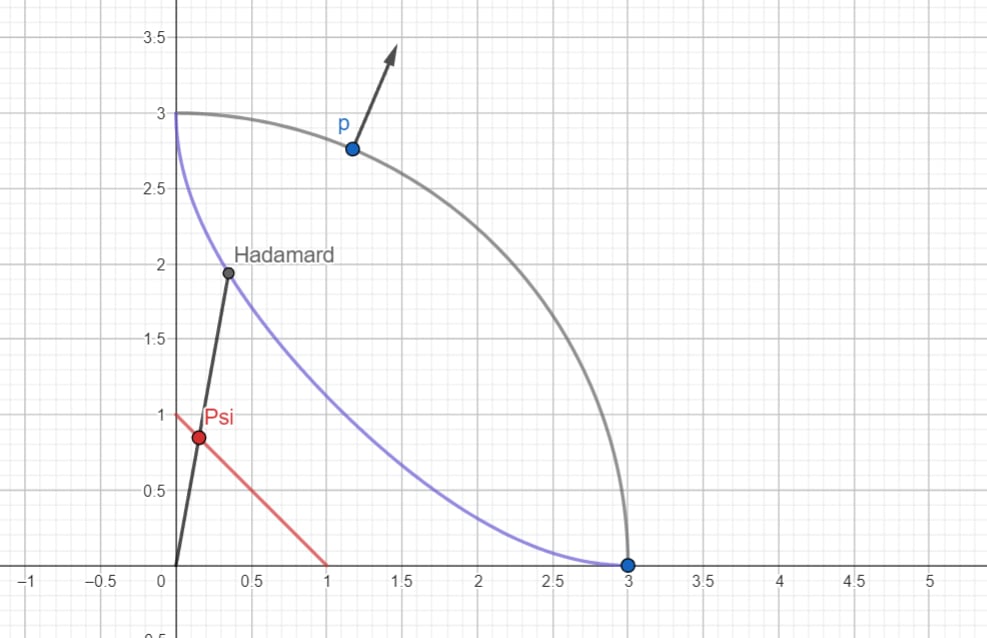
This normalization map $\Delta :\odot (P,\Phi )\to {\Delta }^n$ follows the same pattern as $\odot (P,\Phi )$; in the interior of the Harsanyi Shadow we can uniquely recover $p\odot \varphi$ from $\frac{p\odot \varphi }{p\cdot \varphi }$. And for those points we know we can also uniquely recover $(p,\varphi )$ from $p\odot \varphi$. 

Normalizing the Interior of the Harsanyi Shadow is Injective

Is it possible for two different points on $\odot (P,\Phi )$ to get scaled down to the same point on ${\Delta }^n$? This would require $p\odot \varphi =\lambda (q\odot \tau )$ for some $\lambda \in R^n$, where $(p,\varphi ),(q,\tau )\in (P,\Phi )$. Around the boundary of the Harsanyi Shadow this can happen, but it turns out it can't in the interior!

As we've seen, $\frac{\partial {\varphi }_i}{\partial p_i}\ge 0$, so increasing $p_i$ never decreases ${\varphi }_i$. This means that increasing $p_i$ always increases $(p\odot \varphi {)}_i$ in the interior. (This is the step that fails on the boundary when $p_i=0$ or ${\varphi }_i=0$ for any agent.) But increasing the utility for one agent never increases the feasible utility available for any other agent. $\frac{\partial p_j}{\partial p_i}\le 0$ when $i\ne j$.

This is why the interior of the Harsanyi Shadow doesn't contain any points on the same line from the origin. Moving from $(p,\varphi )$ to $(q,\tau )$ would involve simultaneously increasing (or simultaneously decreasing) $(p\odot \varphi {)}_i$ for all agents. But increasing $p_i$ for one agent, and thus $(p\odot \varphi {)}_i$, must monotonically decrease $p_j$ for all other agents, and thus monotonically decrease $(p\odot \varphi {)}_j$. And similarly, decreasing $p_i$ never decreases $(p\odot \varphi {)}_j$ in the interior.

Normalizing the Harsanyi Shadow is Surjective

Given $\psi \in {\Delta }^n$, can we always find $(p,\varphi )\in (P,\Phi )$ such that 

$\psi =\frac{p\odot \varphi }{p\cdot \varphi }$

This one is pretty straightforward: $G(\_,\psi )$ always has some optima, and at least one of them will be a point $p\in P$ which is consistent with a $\varphi \in {\Delta }^n$ that satisfies this equation. Because that's the "find $\psi$ to make $p$ optimal according to $G(\_,\psi )$" equation.

Geometrically, this tells us that the Harsanyi Shadow of $P$ doesn't have any holes. If we draw a line from the origin through $\psi$, it will hit the Harsanyi Shadow somewhere.

Moving Continuously Across the Harsanyi Bundle

Putting it all together, in the first part of this sequence we started by computing the weights $\psi$ which would make a chosen point $p\in P$ optimal according to $G(\_,\psi )$. We formalized that here by choosing a point $(p,\varphi )\in (P,\Phi )$, computing their Hadamard product $p\odot \varphi$, then scaling this down to land on ${\Delta }^n$.

$\psi =\frac{p\odot \varphi }{p\cdot \varphi }$

$(P,\Phi )\to \odot (P,\Phi )\to {\Delta }^n$

Going in the reverse direction, we can draw a line from the origin through $\psi$ to a find where that line intersects the image $\odot (P,\Phi )$, which we've been calling the Harsanyi Shadow. If $\psi$ is in the interior of ${\Delta }^n$, where ${\psi }_i>0$ for all agents, this point $p\odot \varphi$ on the interior of the Harsanyi Shadow is unique! And from there we can uniquely recover the point $(p,\varphi )$ in the interior of the Harsanyi Bundle, such that $p$ is optimal according to $G(\_,\psi )$ and $H(\_,\varphi )$.

In this last section, I want to describe the challenge of extending this continuity result to include weights $\psi$ where at least one agent has $0$ geometric weight, and some ways of addressing that challenge.

The Challenge of Continuity Around the Boundary

We've called the weight-derivation function $\psi (p,\varphi )$, so let's call the inverse ${\psi }^{-1}\left(\psi \right)$, which corresponds to maximizing $G(\_,\psi )$ and breaking ties around the boundary somehow. Ideally, we would like this function to be continuous, so that individual utilities shift continuously as geometric weights shift. In order for that to be true, ${\psi }^{-1}$ needs to be equal to its limit points everywhere.

${\psi }^{-1}\left(\psi \right)=\underset{\sigma \to \psi }{lim}{\psi }^{-1}\left(\sigma \right)$

We have a bijection between the interiors of ${\Delta }^n$ and $(P,\Phi )$, between weights $\psi$ where ${\psi }_i>0$ for all agents and pairs $(p,\varphi )$ where $p_i>0$ and ${\varphi }_i>0$ for all agents. And so my first hope was that we could take the limit as we approach the boundary, to define the value at every point along the boundary. Unfortunately, this limit depends on how we approach corner points, in a way that makes me suspect that there's no way to way to inherit values for ${\psi }^{-1}$ around the boundary, in a way that simultaneously

• Agrees with $\underset{u\in F}{\arg max}G(u,\psi )$ exactly on the interior
• Leads to ${\psi }^{-1}$ being continuous when its domain includes the boundary

Motivating Example

When multiple agents have $0$ weight according to $\psi$, there can be many Pareto optima that maximize $G(\_,\psi )$. For example, suppose that Alice is a $G(\_,\psi )$ maximizer deciding how much money she should receive, from $0-$100. And simultaneously, how to split another $100 between Bob and Carol. Conveniently, they each derive utility equal to the money they receive.

When trade-offs are linear, maximizing $G(\_,\psi )$ splits utility between agents proportionally to their weight. In particular, when an agent receives a vanishingly small, but positive, share of the geometric weight ${\psi }_i$, they receive a vanishingly small, but positive share of the utility $u_i$.

In this example, let's say that Alice assigns herself ${\psi }_{Alice}=\alpha$. The claim I'll be making is that in this example, we can't satisfy those two desiderata from the previous section. We can't extend ${\psi }^{-1}$ exactly in a way that makes it continuous.

To see why, let's first consider what happens if Bob receives a vanishingly small weight ${\psi }_{Bob}=ϵ$, and Carol receives the remaining weight ${\psi }_{Carol}=1-\alpha -ϵ$. If we take the limit as $ϵ$ approaches 0, $u_{Bob}$ approaches $\$0$ and $u_{Carol}$ approaches $\$100$.

What if the roles are swapped, so that ${\psi }_{Carol}=ϵ$, and Bob gets the rest of the weight ${\psi }_{Bob}=1-\alpha -ϵ$? Then if we take the limit as $ϵ$ approaches $0$, $u_{Bob}$ approaches $\$100$ and $u_{Carol}$ approaches $\$0$.

So along one boundary of ${\Delta }^n$, if we inherit values according to the limit as we approach the boundary, $u_{Bob}=\$0$ and $u_{Carol}=\$100$ because ${\psi }_{Bob}=0$ and ${\psi }_{Carol}>0$. And along another boundary, $u_{Bob}=\$100$ and $u_{Carol}=\$0$ because  ${\psi }_{Bob}>0$ and ${\psi }_{Carol}=0$.

What happens at the corner where these boundaries meet, where ${\psi }_{Bob}=0$ and ${\psi }_{Carol}=0$? No matter what value we assign, ${\psi }^{-1}$ must jump discontinuously here. And in fact, we can reach any split between Bob and Carol by approaching on different paths that preserve different ratios between their vanishingly small weight. (Equal weight gets them an equal split, a 60:40 ratio of weight gets them a 60:40 split of the money, and so on.)

The issue is that maximizing a weighted average, whether a linear average like $H(\_,\varphi )$ or a geometric average like $G(\_,\psi )$, really does treat $0$ weight differently from a small but positive weight $ϵ$. A positive weight makes the weighted average sensitive to increases in an agent's utility, even if only a little bit. But there can be an arbitrarily huge difference between "the payoff Bob receives if Alice assigns him $0$ weight" and "the payoff Bob receives if Alice assigns him some tiny amount of weight."

How to Achieve Continuity Anyway

So it seems like in order to achieve continuity, we need to do one of the following:

• Ensure that ${\psi }_i>0$ for all agents
• Maximize something other than $G(\_,\psi )$

One way to take that second approach would be to derive new weights $\beta \left(\psi \right)$ and then maximize $G(\_,\beta (\psi \left)\right)$. If ${\beta }_i>0$ for all agents, no matter what weights $\psi$ we started with, then we can use all that work we did in this post to show that $G(\_,\beta (\psi \left)\right)$ has a unique optimum that travels continuously around $P$ as we change $\beta$. If $\beta \left(\psi \right)$ is continuous, then so is ${\psi }^{-1}\left(\psi \right)$.

${\psi }^{-1}\left(\psi \right)=\underset{u\in F}{\arg max}G(u,\beta (\psi \left)\right)$

Ideally, we'd like $\beta$ to be very close to $\psi$, while assigning all agents positive weight. One way to do this is to pick a very small amount of weight $ϵ$, and scale $\psi$ down so that ${\sum }_{i=1}^n{\psi }_i=1-ϵ$. Then we can distribute that small weight $ϵ$ equally among all $n$ agents, giving them a minimum weight of ${\beta }_i=\frac{ϵ}{n}$

${\beta }_i={\psi }_i(1-ϵ)+\frac{ϵ}{n}$

This ensures that the sum of weights ${\sum }_{i=1}^n{\beta }_i$ is still 1. We can pick $ϵ$ to be arbitrarily small, making the difference $\beta -\psi$ arbitrarily small. If all we want is a tie-breaker, and we don't care about continuity, we can take the limit as $ϵ$ approaches 0.

${\psi }^{-1}\left(\psi \right)=\underset{ϵ\to 0}{lim}\underset{u\in F}{\arg max}G(u,\beta (\psi ,ϵ\left)\right)$

But for the applications I have in mind, I actually prefer continuity even if it means requiring a minimum positive weight for all agents. In terms of morality, that seems like a feature rather than a bug. It seems like the kind of feature that might get a superintelligent AI to leave us the Milky Way, even if it seizes the rest of the observable universe for its own misaligned ends.

Anything we deem an "agent" probably does deserve some positive weight in our utility aggregation function. This particular formula is inspired by moral reasoning along the lines of "reserve a small amount of weight $ϵ$ and distribute it equally among all agents, regardless of any other considerations like their ability to reciprocally benefit the decision-maker."

So my current favorite approaches involve always assigning agents positive weight when it comes to $G(\_,\psi )$ maximization. Which might look like designing the weight-attribution function so that it's always positive, or it might look like padding $\psi$ so that every agent has positive weight as far as $G(\_,\psi )$ is concerned.

1. ^{^}

   This function isn't defined when $p\cdot \varphi =0$, but in this case the entire feasible set $F$ is a single point at the origin. And indeed in this case, any reconstruction function will look like $p(\psi ,\{\overrightarrow{0}\left\}\right)=\overrightarrow{0}$, which is continuous!

2. ^{^}

   For topological spaces in general, the inverse of a continuous bijection isn't necessarily continuous.

3. ^{^}

   The tangent space for a manifold isn't always a hyperplane. For example, consider a circle embedded in 3-dimensional space; each tangent space is still just a line. This section is the reason we assumed $F$ is $n$-dimensional (there aren't any redundant players with constant utility), so that $P$ is an $n-1$ dimensional hypersurface with tangent hyperplanes.

4. ^{^}

   All of the convex combinations within ${\Delta }^n$ anyway. Some faces can be oriented so that if you try calculating $\varphi$ for them, you end up with ${\varphi }_i<0$ for some agent. These faces are Pareto dominated, and when calculating the valid values of $\varphi$ at a corner we can ignore convex combinations that extend beyond ${\Delta }^n$.

5. ^{^}

   At least the interior of this surface is an $n-1$ dimensional manifold. I haven't proven or disproven whether the whole Harsanyi Bundle is a manifold, but I suspect it is. $P$ is an $n-1$ dimensional manifold, and so is ${\Delta }^n$, but in order for $(P,\Phi )$ to be a manifold, it needs to always stay $n-1$ dimensional and never fork or collapse down to a lower number of dimensions.

0 comments

Comments sorted by top scores.