Logical induction for software engineers

post by Alex Flint (alexflint) · 2022-12-03T19:55:35.474Z · LW · GW · 8 comments

Contents

  Outline
  Motivation
  Credences on binary-valued variables
    Terminology and type signatures
  Type signature of a logical inductor
    Terminology and type signatures
  The logical induction criterion
    Terminology and type signatures
    Comparison to probability theory
    Consequences of satisfying the logical induction criterion
  The logical induction algorithm
    Defeating one trading algorithm
    Defeating multiple trading algorithms
    Defeating all possible trading algorithms
    Deciding which sentences to put credences on
    Summary of the algorithm
  Summary of terminology and type signatures
  Conclusion
  Appendix: Worked example
    Install the logicalinduction package
    In the code below we will work with these 3 sentences:
    First we create a helper function that builds trading formulas
    Let's plot the quantity traded by this formula as a function of price
    Now we define a trading algorithm
    Create a logical inductor and perform two updates
    Let's look at the inner workings of the logical induction algorithm
    Now we solve for our a belief state where this trading policty makes very few trades
    Plot the space over which find_credences searches
    Compute a budget factor
None
8 comments

This work was supported by the Monastic Academy for the Preservation of Life on Earth and the Long Term Future Fund.

Outline

• This post is an explanation of the theory of logical induction developed by Garrabrant et al
• I formulate the theory in a way that should make sense to software engineers and those with a software engineering mindset.
• I will go through a full implementation of the logical induction algorithm in Python, and I will use it to explain the basic theory of logical induction, including the core logical induction algorithm.
• I will give type signatures for all concepts and will work through all algorithms in terms of a sequence of processing steps.
• The Python code for this guide is here.
• The Colab notebook for this guide is here.
• The index of type signatures for this guide is here.

Motivation

Logical induction is a theory, published in 2016 by Scott Garrabrant, Tsvi Benson-Tilsen, Andrew Critch, Nate Soares, and Jessica Taylor, about how to build machines that maintain uncertainty about the world and update those beliefs in light of evidence. It does this by assigning numbers between 0 and 1 to claims about the world, just as probability theory does, but it makes different guarantees about the internal relationship between those numbers. Whereas probability theory guarantees that its numbers will obey the sum and product rules of probability, logical induction guarantees that the evolution of its numbers over time will obey the logical induction criterion.

Many people have heard that logical induction is about having uncertainty in purely logical facts. It is true that logical induction shows how to construct algorithms that maintain uncertainty in purely logical facts, but in my view this is not really the point of logical induction. The point of logical induction, in my view, is that it is always computable, even when reasoning about contradictory, uncomputable, or self-referential questions. Its capacity to maintain uncertainty about purely logical facts is actually a by-product of the computability of logical induction.

Logical induction addresses the same basic problem that probability theory addresses. Logical induction and probability theory, therefore, are two different answers to the question: what is a reasonable formal method for quantifying uncertainty and updating it in light of evidence? Probability theory and logical induction both provide concrete operationalizations of "quantified uncertainty" (henceforth "credence"), and what it means for a set of credences to be "reasonable".

Probability theory says that credences are "reasonable" if it is impossible for someone to bet against you in a way that is expected to make money, independent of the true state of the world (a Dutch book). Logical induction says that credences are "reasonable" if it is impossible for someone to bet against you in a way that makes more and more money over time with no corresponding down-side risk. The probability theory formulation is the stronger guarantee; its drawback is that it is not in general computable. The logical induction formulation is computable, and in this guide we will walk through a general purpose algorithm for computing credences given complicated, even self-referential, world models.

At its core, the theory of logical induction consists of two things:

1. A set of proofs showing that if you assign credences in a way that is consistent with the logical induction operationalization of uncertainty then your credences are guaranteed to exhibit certain common-sense desirable properties such as consistency over time, unbiasedness over time, converging to well-calibrated limits in a timely manner.

2. An algorithm that assigns credences in a way that is consistent with the logical induction operationalization of uncertainty. The existence of this algorithm establishes that the logical induction operationalization of uncertainty is computable. This is the algorithm that we will work through in this guide. It is extremely inefficient.

A by-product of the computability of logical induction is that logical induction propagates logical uncertainty gradually, rather than all at once as in probability theory. What this means is that the logical induction algorithm, upon receiving an observation, may not propagate the logical consequences of those observations to all of its credences immediately. For example, if you tell a logical inductor that two variables X and Y are highly correlated, and then you further update your logical inductor with the actual value of X, then the logical inductor may not immediately come to the logical conclusion concerning the possible values of Y:

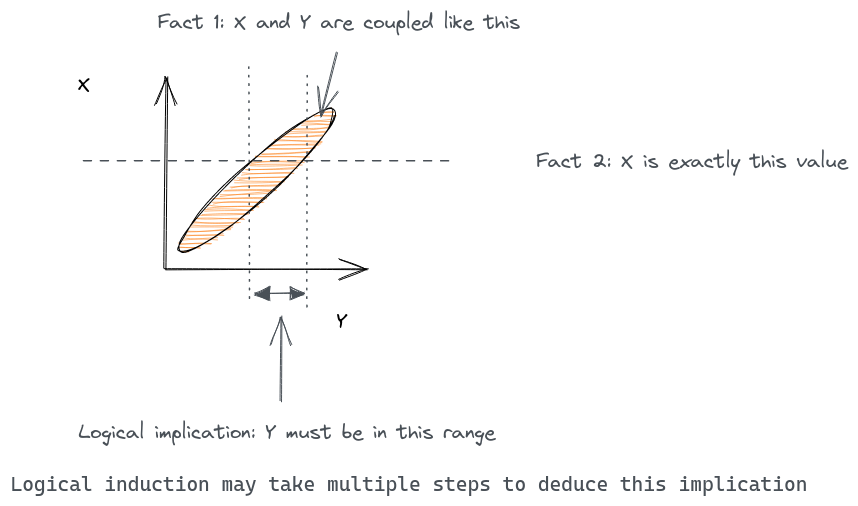
Any computable algorithm for updating uncertainties over time must propagate logical consequences step-by-step rather than all-at-once, because propagating all the logical consequences of an observation is uncomputable in general, since we might have a world model where knowing the logical consequences of an observation is equivalent to knowing something uncomputable (e.g. whether some Turing machines halts or not). Therefore the ability of logical induction to maintain uncertaint about purely logical facts is really just a by-product of the more general feature of being a computable method of updating well-calibrated credences in light of evidence.

When we say that "logical induction is computable" we mean that there exists an algorithm that implements the logical induction operationalization of uncertainty for full-general models. There is no such fully-general algorithm for probability theory.

The remainder of this document is organized as follows. First we will look at how we can reduce everything to credences on binary-valued variables with logical relationships between them. Next we look at the inputs and outputs to the logical induction algorithm and their type signatures. Then we discuss the logical induction criterion, which you could view as the "spec" for the logical induction algorithm. Then we go through the logical induction algorithm itself in detail. Finally, we will review a worked example in the form of a Jupyter notebook.

Credences on binary-valued variables

In classical treatments of probability theory, everything starts with probabilities on binary-valued variables, and probabilities on continuous variables are built up out of that.

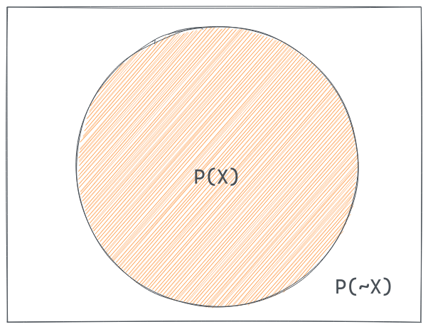
For many of us, though, it is more common to think directly in terms of continuous variables with probability distributions over them:

In logical induction, everything is worked out in terms of binary-valued variables, and all relationships between variables are written in the language of first-order logic, which means combinations of AND, OR, NOT, FOR-ALL, and THERE-EXISTS relationships. The first task in applying logical induction to any problem is to formulate that problem in terms of binary-valued variables with purely logical relationships between them. This could be done in any number of ways, such as:

• To talk about a continuous-valued variable x with a fixed distribution (say a Gaussian distribution with some particular mean and variance) you could have a set of binary-valued variables $X_a$, each of which is true whenever the the continuous-valued variable is less than $a$. Logical induction does not "see" the value of $a$ in $X_a$ --- it just "sees" an undifferentiated binary-valued variable whose truth depends logically on some other variables.

• To talk about two continuous-valued variables x and y that are correlated, you could construct a third continuous-valued variable $z$ representing the deviation of $x$ and $y$ from perfect correlation, and then construct three sets of binary-valued variables $X_a$, $Y_b$, and $Z_c$ as per the previous bullet point. You would add logical relationships of the form "IF $X_a$ AND $Y_b$ THEN $Z_c$" for the particular values of $a$, $b$, and $c$ corresponding to the correlation coefficients between $x$ and $y$. That is, if it was the case that $z=y-x$ then we would feed logical induction the sentence "IF $X_2$ AND $Y_9$ THEN $Z_7$" (because $7=9-2$) along with other multiples of these coefficients

• To talk about a computer program, we might have a binary-valued variable for each possible value of each variable after executing each line of code. The lines of code would then become logical relationships between those variables.

You may be concerned at this point that there are an infinite number of binary-valued variables that we need to track, and an infinite number of constraints between them. The way we deal with this in logical induction is by feeding the constraints into the logical inductor as "observations", one-by-one, such that at every point in time the logical inductor has only a finite number of sentences to deal with. Each one of those finite sentences contains only a finite number of binary-valued variables, so the logical inductor is always working with a finite number of binary-valued variables. The logical induction algorithm does not require any up-front list of all the variables in the world, or anything like that; rather, when it receives a new sentences containing a variable previously unknown to it, it can begin tracking and updating credences in that variable seamlessly.

In the remainder of this document we will refer to a binary-valued variable as an "atom" and to a logical statement about some variables as a "logical sentence". A logical sentence that we pass to our logical inductor as "observed true" will be referred to as an "observation".

Terminology and type signatures

Here is a summary of the concepts introduced up to this point. In the table below (and in similar tables given at the end of each major section of this write-up), the "concept" column contains a term was introduced in the text above, the "type" column contains a type signature, the "in the paper" column contains the corresponding term used by Garrabrant et al in the paper that introduced logical induction, and "In Python code" contains, where possible, a link to the corresponding code in the logical induction repository on Github. Since this is the first such table, the three concepts below all have elementary types. In future tables, many concepts will have types composed of previous types.

Concept	Type	In the paper	In Python code
Credence	Real number	Price	float
Atom	Atom	Atom	class Atom
Observation	Sentence	Sentence	class Sentence

Type signature of a logical inductor

A logical inductor takes in a sequence of observations (sentences) one-by-one, and after processing each one produces a belief state, which is a list of (sentence, credence) pairs, where a credence is a real number between 0 and 1.

At each step, we only put credences on a finite set of sentences, so the list of (sentence, credence) pairs is finite in length. Each time an observation is provided as input, a new belief state is generated as output.

The credences fulfill the same basic purpose as probabilities in probability theory, but they need not obey the laws of probability theory, so we do not call them probabilities. Instead, they obey the logical induction criterion, which is a different notion of what it means to quantify one’s uncertainty about a claim about the world, to be discussed in the next section.

When we feed a sentence into the logical inductor as an observation, we are telling the logical inductor to take that sentence to be true. The logical inductor’s job is then to update its credences in other related sentences. The theory of logical induction is not concerned with how we generate these observations, just as probability theory is not concerned with how we generate the observations that we condition on.

The most important aspect of logical induction to be clear about is that this is a new formalization of what it means to associate numerical credences with claims about the world. Probability theory is one possible formalization of the general phenomena of reasoning about the world by updating credences in response to evidence. The formalization proposed by probability theory is compelling because (in Jaynes’ formulation of probability theory) it arises as the only possible solution to a set of mild desiderata. But it also has a serious drawback in requiring us to compute all the logical consequences of each new observation before we can produce a new belief state consistent with its laws, and the physics of our world does not permit machines that decide the logical consequences of general facts in finite time. Logical induction introduces a different notion of what it means to associate a numerical credence with a claim about the world. It makes a weaker set of guarantees about those credences, but in exchange we get a computable algorithm for updating beliefs in light of new observations^[1].

Terminology and type signatures

Concept	Type	In the paper	In Python code
BeliefState	List<Pair< Sentence, Number >>	Belief state	N/A

The logical induction criterion

The logical induction criterion is the specification that a computer program must meet in order to be deemed a "logical inductor". By analogy, consider a "sorting algorithm criterion" requiring each number in the program’s output to be less than or equal to the next number. There are many different sorting algorithms that meet this criterion; likewise, there are many algorithms that meet the requirements of the logical induction criterion. In the case of the logical induction criterion, we have (in the logical induction paper) a set of proofs showing that if an algorithm meets this specification, then the credences output by the algorithm will be convergent in a certain sense, coherent in a certain sense, unbiased in a certain sense, and so on. It is critical to understand the logical induction criterion because otherwise the logical induction algorithm will make little sense.

The logical induction criterion says that our credences should be set such that if we were to bet on them, there would be no continuous polynomial-time trading algorithm that would take more and more money from us, update after update, without limit, and without downside risk. What this means is that if you give me a computer program and that inputs observations and outputs credences, and I find an algorithm (within a certain restricted class that we will discuss below) that trades against it in a way that makes unboundedly much money, then I have proven that your algorithm does not obey the logical induction criterion. If there is no such trading algorithm then your computer program obeys the logical induction criterion.

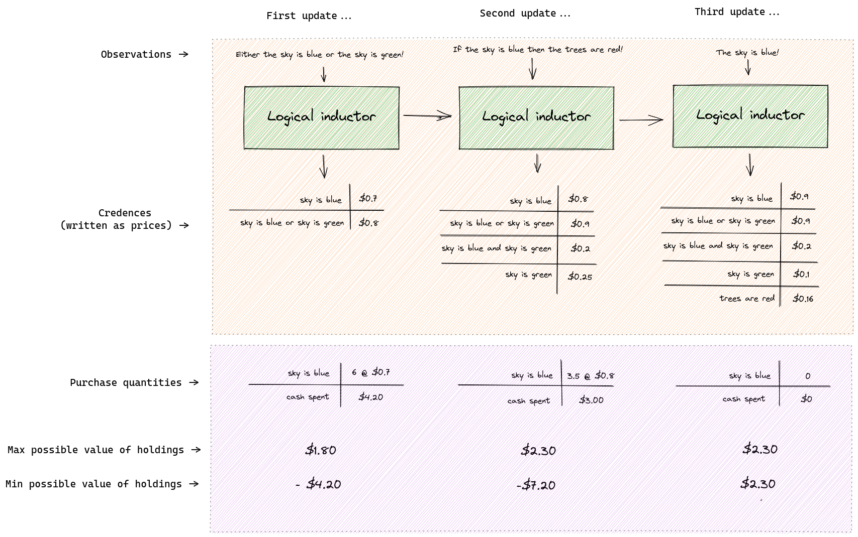
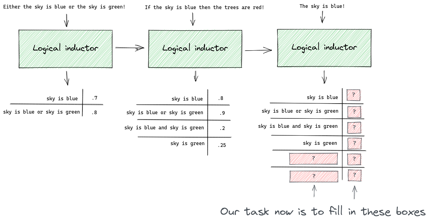
What does it mean to "trade against" a computer program that outputs credences? We interpret each credence as a price for a token that pays $1 if the respective sentence is eventually confirmed as true. So a credence of 0.6 assigned to X means that I am willing to sell you a token for 60c that pays out $1 if X is eventually confirmed as true. What it means to "be confirmed as true" is that X appears in the observation stream. Here is an example with three successive updates and a single trading algorithm that trades against the logical inductor:

Note:

1. The logical inductor’s credences may not immediately reflect its observations. Even though it knows that the sky must either be blue or green on the first day, it still doesn’t assign 100% credence to the sentence "the sky is blue or the sky is green". It is guaranteed to converge to 100% eventually on that sentence, but it may take a while.

2. The logical inductor credences may not immediately be probabilistically consistent. Even though it knows that the sky must either be blue or green, on the second day it assigns 0.8 credence to "the sky is blue" and 0.25 credence to the "the sky is green", which don’t sum to 1. It will converge on credences that sum to 1 eventually, but it may take a while.

3. This example shows trades made by just one possible trading algorithm. I chose the numbers in the "purchase quantities" row arbitrarily.

4. This trading policy only makes trades in one sentence. That is just for simplicity. In general trading policies can make trades in any number of sentences after each update.

5. The last two rows in the figure are calculated as follows.

6. On the first update we spent $4.20 to purchase 6 tokens of "sky is blue". If it turns out that the sky really is blue, then our tokens will be worth $6 ($1 for each of 6 tokens), in which case we will have made a profit of $1.80. If it turns out that the sky is not blue then our tokens are worth $0 and we will have lost $4.20. At this point we have only purchased tokens in this one sentence so the minimum and maximum possible value of our holdings are $4.20 and -$1.80 respectively.

7. On the second update we purchased a further 3.5 tokens of "the sky is blue" for $3.00 ( the price per token for this sentence changed between the first and second update). We now own 9.5 tokens, which could be worth $9.50 if the sky really is blue, in which case we would have made a profit of $2.30. If the sky turns out not to be blue then we will now have lost $7.20. In this example we only purchase tokens in one sentence in order to keep the calculations simple, but in general any number of tokens in any number of sentences can be purchased.

8. On the third update we observe that the sky is blue. When calculating the "min" and "max" rows we only consider possibilities that are logically consistent with what we have observed. Since we own 9.5 tokens of "the sky is blue" and we know now that the sky really is blue, the min and max values become identical at $2.30.

What does it mean to make unboundedly much money? If the maximum possible value of a trading algorithm’s holdings grows larger and larger over time without limit, while the minimum possible value does not become more and more negative without limit, then we say that the logical inductor has been "exploited". Suppose we continued the figure above for many steps and made a graph of the "max possible value of holdings" and "min possible value of holdings". Here are three possibilities for how the numbers could evolve:

In the first figure, the max and min both keep growing unboundedly over time, and this does not meet the definition of exploitation used in the logical induction criterion. In the second figure, the max and min both reach a bound, and this again does not meet the definition of exploitation used in the logical induction criterion. In the third example the max grows unboundedly over time while the min reaches a bound, and this does meet the definition of exploitation used in the logical induction criterion. If there exists any polynomial time trading algorithm with a max line that grows unboundedly and a min line that reaches a bound, then the credences under consideration are exploitable. If there is no such algorithm then our credences are unexploitable and we have satisfied the logical induction criterion.

What is the restricted class of trading algorithms? Logical inductors do not have to be unexploitable versus all possible algorithms, only to a certain restricted class that we will call "trading algorithms". A trading algorithm is a polynomial time computer program that outputs "trading policies". A trading policy is a list of pairs of (sentence, trading formula). A trading formula is a continuous function, built up from six primitives, that inputs a list of lists of (sentence, credence) pairs and outputs a real number representing a quantity of tokens to purchase.

The six trading primitives are:

1. Purchase a constant number of tokens

2. Take the sum of two trading formulas and purchase that many tokens

3. Take the product of two trading formulas and purchase that many tokens

4. Take the max of two trading formulas and purchase that many tokens

5. Take the reciprocal of a trading formulas and purchase that many tokens

6. Look up the credence associated with a sentence and purchase that many tokens

In the code, trading formulas are implemented by Formula.

So the trading algorithms that we must not be exploited by are actually programs that output policies for how much to trade as a function of the price of various sentences:

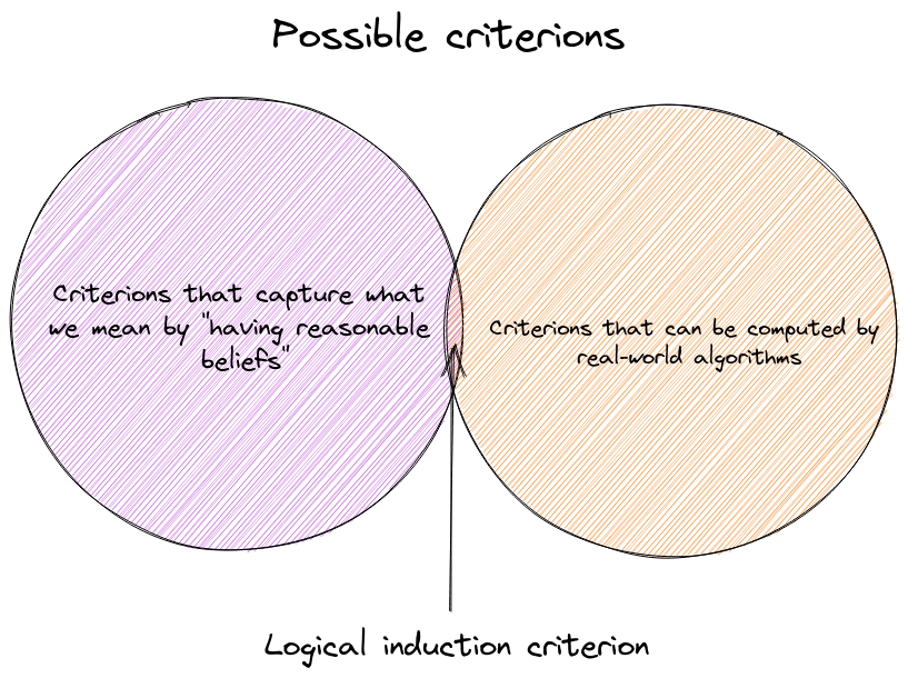
The restriction in which trading algorithms must output policies, rather than directly performing trades, is crucial to making the whole logical induction system work. If we allowed trading algorithms to directly output trades then the problem of finding unexploitable credences would be so difficult that there would be no real-world algorithm that accomplishes it, because we would be asking for a computer program that systematically outsmarts every possible computer program. In this way the logical induction criterion threads the needle between capturing much of what it means to update beliefs in light of evidence, while permitting a real-world algorithm that satisfies it. This is really the crucial discovery in the whole theory of logical induction:

Terminology and type signatures

Here is a summary of the type signatures of the concepts we have introduced in this section

Concept	Type	In the paper	In Python code
BeliefHistory	List<BeliefState>	Belief history	class History
Price, Constant, Sum, Product, Max, Reciprocal	Function: PriceHistory -> List<Pair< Sentence, Number	Expressible feature	class Price class Constant class Sum class Product class Max class Reciprocal
TradingPrimitive	Price	Constant	Sum
TradingFormula	TreeOver<TradingPrimitive>	Expressible feature	class Formula
TradingPolicy	List<Pair< Sentence, TradingFormula >>	Trading strategy	N/A
TradingAlgorithm	Generator<TradingPolicy>	Trader	N/A

Comparison to probability theory

The formulation of probability theory given by E. T. Jayes also took the shape of a criterion and a solution to that criterion. Jaynes’ criterion was that one’s credences ought to be numerical, consistent with certain common-sense inequalities, and independent of the order in which one updates on different pieces of information. Jaynes showed that the only way of satisfying this criterion was via the sum and product rule of probability theory. This is such a strong result that it seems, from a certain perspective, to completely settle the question of how one ought to quantify and update one’s beliefs in light of evidence. However, the sum and product rules of probability theory are not computable in general! The reason is that one can set up arbitrarily complicated logical relationships between variables in such a way that evaluating the sum and product rule is equivalent to determining whether certain computer programs halt or not, which is uncomputable.

In statistical learning theory it is actually rather rare to formulate a statistical problem in which the sum and product rule can be evaluated exactly. Instead, an approximation algorithm is used, and as a result there is a separation between the theory concerning what one ought to compute (probability theory), and the theory concerning how to approximate that (some particular approximation algorithm and its guarantees). We rarely get strong guarantees about how the two will behave over time as a sequence of observations are processed, given finite computing resources. From this perspective, logical induction provides a unified theory about both parts of this equation (what to compute and how to compute it; the"gold standard" and the approximation technique). Logical induction says: follow this computable method for generating credences and the sequence of your belief states over time will have such-and-such nice properties. Of course, logical induction is at present highly impractical due to its very high time complexity. However, it may point the way towards something that is actually more practical than probability theory, even in cases where logical uncertainty itself isn’t the main goal.

Another way of looking at the connection between probability theory and logical induction is that in probability theory, we require that each individual belief state be unexploitable on its own (the "no dutch book" notion), whereas the logical induction criterion requires that the sequence of belief states not be exploitable unboundedly over time. That is, the logical induction criterion makes no guarantees about any one belief state, but instead about the evolution of belief states over time.

Consequences of satisfying the logical induction criterion

One of the main contributions of the logical induction paper is a set of proofs showing that if a computer program produces credences obeying the logical induction criterion then those credences are guaranteed to be "reasonable" in the following ways:

1. Convergent. Over time, one’s credences always converge to a single value (Theorem 4.1.1 in the paper)

2. Coherent. Over time, one’s credences eventually become consistent with the sum and product rules of probability theory (Theorem 4.1.2 in the paper)

3. Efficient. If there is an efficient deduction algorithm that eventually proves (or disproves) a sequence of sentences, then one’s credences will converge to 1 (or 0) for all sentences in that sequence within finite time (Theorem 4.2.1 in the paper)

4. Persistent. If one’s credences are going to reflect a certain insight in the limit, then that insight will reflected in one’s credences after a finite amount of time (Theorems 4.2.3 and 4.2.4 in the paper)

5. Calibrated. If one’s credences converge to p for all sentences in some set of sentences, then roughly p% of those sentences will turn out to be true (Theorem 4.3.3 in the paper)

6. Unbiased. For certain well-behaved sequences of sentences, there is no efficient method for detecting a predictable bias in one’s credences (Theorem 4.3.6 and 4.3.8 in the paper)

7. Statistically competent. When faced with a sequence of unpredictable sentences of which p% are true, one’s credences in the entire sequence convert to p (Therems 4.4.2 and 4.4.5 in the paper)

8. Logically competent. The sum of credences over sets of sentences among which exactly one sentence must be true converges to 1 (Theorem 4.5.1 in the paper)

9. Non-dogmatic. One’s credences will only converge to 1 for things that are provably true, and to 0 for things that are provably false (Theorems 4.6.2 and 4.6.3 in the paper). In other words, if something is not provably true then its credence will not converge to 1, and if something is not provably false then its credence will not converge to 0.

These properties are actually extremely subtle in their precise definition. For a full description, see the logical induction paper, section 4.

Each of these definitions talks about the behavior of one’s credences over time. Two important mathematical facts about logical inductors are that (1) if you take a logical inductor and overwrite its credences for the first finitely many updates with any credences whatsoever then it will remain a logical inductor (i.e. will still satisfy the logical induction criterion), and (2) if you overwrite a logical inductor’s credences with the limits to which its own credences would have converged, then it is not a logical inductor (i.e. will not satisfy the logical induction criterion). These two points show that logical induction is neither about the "early" (first finitely many) credences, nor about the "final" (limiting value of) credences, but about the behavior of credences over time.

The logical induction algorithm

Suppose now that you are a logical inductor. Some observations have been fed to you, and you have generated in return some belief states. You have just received a new observation, and you are contemplating how to update your credences.

You must answer two questions:

• Which sentences should I include in the list?

• Which credences should I report for each sentence?

We will answer these question in four steps:

• First we will go through an algorithm that answers the second question in the case that there is just one trading algorithm that we are trying not to be exploited by.

• Next we will show how to combine multiple trading algorithms into one, in such a way that we can apply the previous algorithm to get credences that are not exploited by any of the constituent trading algorithms.

• Next we will discuss how to not be exploited by any possible trading algorithm by enumerating all possible trading algorithms one-by-one.

• Finally we will discuss the first question.

Defeating one trading algorithm

Suppose now that your task is not to defeat all possible trading algorithms as required by the logical induction criterion, but just to defeat one particular trading algorithm for which you are given the source code. Defeating a trading algorithm means that we set our credences such that the trading algorithm, through buying and selling tokens from us, does not make an unlimited amount of money. More precisely, it means that either the "min possible value" line gets more and more negative without a lower bound, or the "max possible value" reaches an upper bound, or both. Or in yet other words, it’s fine for the trading algorithm to make money from us for a little while, but we must eventually limit its exploitation such that the value of its holdings are held below some upper bound.

One way to make sure that this trading algorithm does not make unlimited money from us is to set our credences such that, each time it trades with us, it either:

• purchases tokens from us and the price for those tokens is $1, or

• sells tokens to us and the price for those tokens is $0, or

• chooses not to buy or sell any tokens from us at all

(What it means for a trading algorithm to "sell" tokens to us is that it purchases a negative number of tokens of some sentence, which means that we pay it at the time of purchase, and it pays us the $1 per token if the sentence is confirmed as true.)

If a trading algorithm only purchases tokens from us at $1 or sells to us at $0 or makes no trades at all then it will certainly not make any money from us. This is not the only way to limit the amount of money this trading algorithm makes, but it is one way, and if it’s possible to do it this way then it will certainly satisfy the logical induction criterion. One central result in the logical induction paper is a demonstration that this is indeed always possible. The proof of this uses Brouwer’s fixed point theorem, and there is a further proof showing that we can efficiently find a good approximation to this fixed point using a brute force search. These proofs make use of the fact that trading algorithms must output restricted trading policies in order to trade, and that the constituent trading formulas are continuous as a function of credences, and can be further broken down into the six trading primitives. This is why the trading policies are restricted in the way that they are: in order to make this proof possible.

The algorithm for finding credences is actually incredibly simple: we just enumerate all possible rational-valued belief states! For each one, we evaluate the trading policy that we are trying not to be exploited by, to find out what quantity of tokens it would buy or sell at the prices implied by the belief state. Then we calculate the "max possible value of holdings" number discussed above for this one trade, and if it is less than a certain tolerance then we output the belief state. The tolerance starts at $1 for the first update, then $0.50 for the second update, then $0.25, and so on, so that the sum of all the "max possible value of holdings" numbers stays under $2 over all time. This sum represents the "best case" from the perspective of the trading algorithm, or the "worst case" value from the perspective of the logical inductor, because the logical inductor is trying to set credences so that the trading algorithm never makes very much money. By keeping this number under $2 we ensure that this particular trading algorithm does not meet the requirements of "exploitation" discussed above. The fixed-point proof guarantees that there is some belief state that holds the "max possible value of holdings" number to zero, and the approximation proof guarantees that we can find a rational approximation that is close enough to meet the schedule of decreasing tolerances.

The following diagram depicts the search space over which we search in the case that our belief state contains credences for just two sentences. If there are more sentences in our belief state then the search space has a larger number of dimensions.

In the code, the function that implements this algorithm is here. The main loop that runs the search is here, the loop that calculates the "max possible value of holdings" is here, and the tolerance check is here. In the first update we set a tolerance of ½, then in the second update a tolerance of ¼, then ⅛, and so on, such that the all-time sum is never larger than 1. The code that sets this tolerance schedule is here.

You will notice at this point how vastly inefficient the logical induction algorithm is. The number of belief states we may need to try grows exponentially with the number of sentences, and, separately, exponentially with the number of updates that we’ve previously performed, since the tolerance gets tighter with each iteration. For each belief state we then consider a number of possible worlds that also grows exponentially with the number of sentences in order to calculate the "max possible value of holdings". There is then a further exponentially growing inner loop caused by the way that we combine multiple trading policies into one, described below. The logical induction algorithm described here is therefore at least thrice-exponential in the number of sentences, and this doesn’t even consider the slow enumeration of possible trading algorithms discussed two sections below.

Defeating multiple trading algorithms

Consider now the problem of selecting a set of credences that are not exploited by any one of some fixed set of trading algorithms. As in the previous section, we may assume that we are given the source code for the trading algorithms.

The basic idea here will be to combine a finite number of trading policies into an "ensemble trading policy" in such a way that if we are not exploited by the ensemble trading policy, then we are not exploited by any of its constituents. To construct this ensemble trading policy, we apply a transformation to each of the trading policies that holds it to a certain budget, which is a lower bound on "min possible value of holdings". This transformation ensures that the trading policy does not lose more than a certain amount of money in any possible world. In the diagram below, trading formulas are represented as trees of trading primitives.

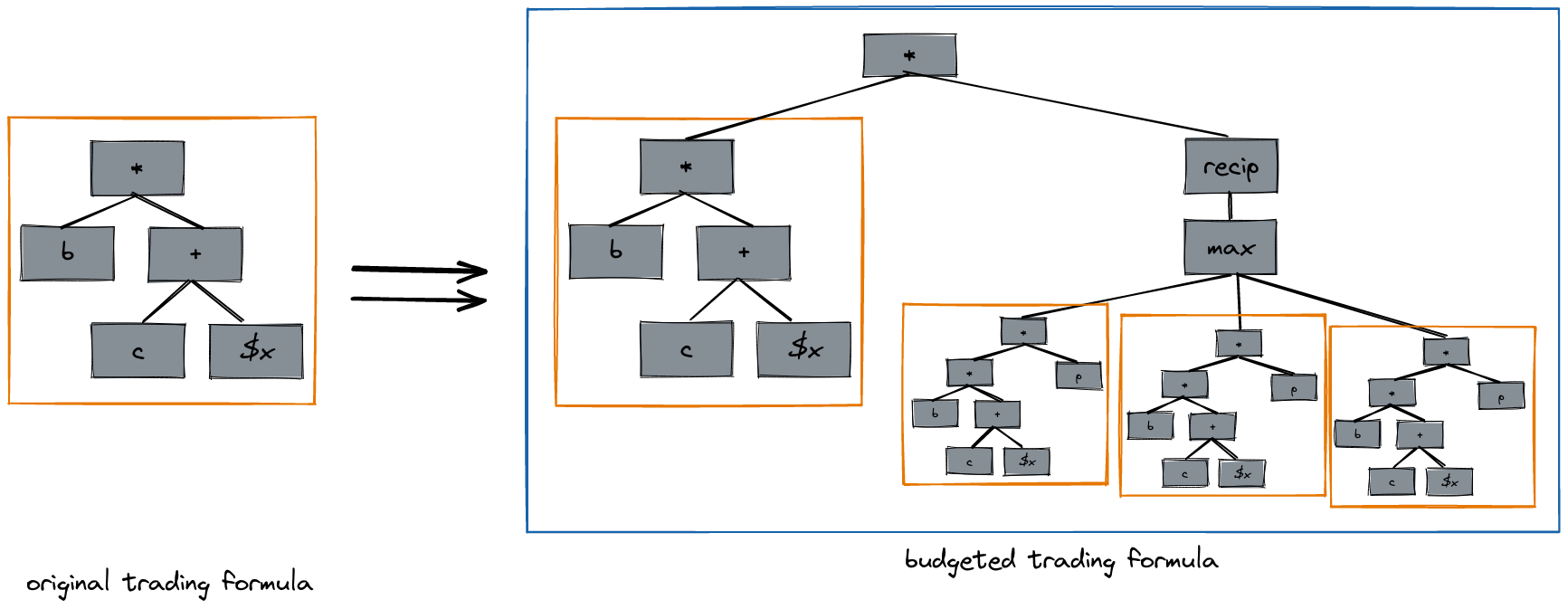
A side note: the budget transform involves pasting the original trading formula multiple times into the output trading formula, and the number of times that the input trading formula is pasted grows exponentially with the number of sentences under consideration by the logical inductor.

The code that applies this budget transform is here. The most intricate part of the whole logical induction algorithm is the code to compute the denominator in the budget transform, which is here. Interestingly, this is the only place that the logical induction algorithm is informed by the rules of propositional logic, which happens here.

Having transformed our trading policies in this way, we combine the trading policies from our different trading algorithms together in a big weighted sum. This weighted sum consists of the trading policies from our N different trading algorithms, each budgeted with multiple different budgets. We can visualize the N trading algorithms as rows in a matrix and budgets of $1, $2, $3 as the columns:

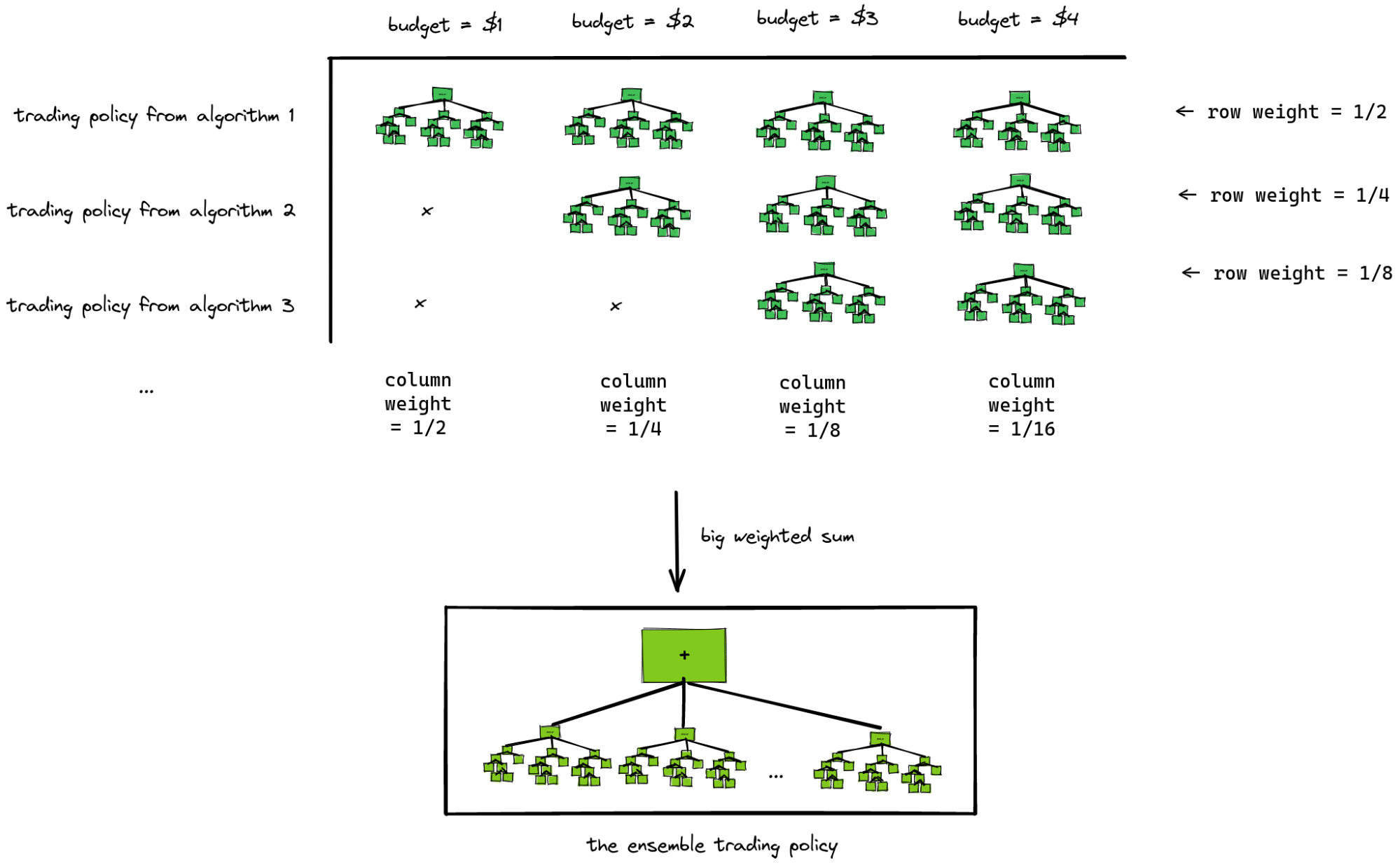
The weight for each cell in this matrix is a product of the row weight and the column weight. Note that while the budgets increase linearly, the weights decrease exponentially. Note also that the entries in each cell in the matrix are trading formulas, and when we "add" them together we are actually combining them into a larger trading formula which contains a symbolic "+" node that evaluates each of the constituent trading formulas and adds their output together.

The reason the budgeting transformation is necessary is that if we had one trading policy that was very smart and one that was very stupid and we simply added them together, then the losses of the stupid policy might eclipse the gains of the smart policy to such an extent that a belief state that avoids exploitation by the combination of the two algorithms may not necessarily avoid exploitation by the smart policy alone. Instead of this, the "budget transform" ensures that the stupid policy will eventually be curtailed, leaving only the smart policy active within the ensemble, which in turn means that the belief state will have to contend directly with the smartest policies in the ensemble.

The code that combines multiple trading policies into one is here. The loop over the rows in the table depicted above is here, and the loop over columns is here. In the end we get the ensemble trading policy here, which we pass to the algorithm described in the previous section here.

Defeating all possible trading algorithms

In order to not be exploited by any polynomial time trading algorithm, we actually just enumerate all possible trading algorithms by directly enumerating turing machines, adding one more element from this enumeration to the ensemble before each update. On the very first update, therefore, we produce a belief state that is only guaranteed not to be exploited by one particular trading algorithm (whichever happens to be the first in this enumeration). Then, on the second update, we add one further trading algorithm to the ensemble, and produce a belief state that is guaranteed not to be exploited by either of these two trading algorithms. Eventually any particular trading algorithm will appear in this enumeration, and after that the logical inductor will output belief states that are not exploited by that trading algorithm. Therefore any trading algorithm whatsoever can only exploit the logical inductor for finitely many steps.

In the code, the next trading algorithm is actually an input to the function that computes updates, because any real implementation of an enumeration of all turing machines would make any testing whatsoever completely impractical. In my testing I set up enumerations of trading algorithms that put the most interesting trading algorithms first, such as here.

Deciding which sentences to put credences on

At each update we have a finite number of trading algorithms, each of which generates a trading policy, each of which contains a table of (sentence, trading formula) pairs, and each trading formula is a tree that looks up credences for some finite number of sentences. We take the union of all the sentences referenced in the trading policy tables (the sentences that the trading policies will attempt to trade on) together with all the sentences referenced within any of the trading formula trees (the sentences whose prices affect the behavior of the trading policies) as the set of sentences to place credences on.

What this means is that we are leaving it to the user to decide in what order to enumerate all the possible trading algorithms, and using that ordering to determine which sentences to place credences on at which time.

There is no need to place credences on sentences that aren’t used as inputs to a trading formula and aren’t traded on by any trading policy, because credences in these sentences wouldn’t affect anything. Our goal at each step is to find a set of credences that cause the current ensemble trader to trade very little, and in order to do this it makes sense to only consider the sentences that affect the current ensemble trader’s behavior or holdings.

Summary of the algorithm

In block diagram form, the process for generating a set of credences for a single update looks like this:

Here are links to the code for the functions referenced in monospace font in the figure above:

• LogicalInductor.update

• compute_budget_factor

• combine_trading_algorithms

• find_credences

Summary of terminology and type signatures

Concept	Type	In the paper	In Python code
Credence	Real Number	Price	float
Atom	Atom	Atom	class Atom
Sentence	Sentence	Sentence	class Sentence
BeliefState	List<Pair< Sentence, Number >>	Belief state	N/A
BeliefHistory	List<BeliefState>	Belief history	class History
Price Constant Sum Product Max Reciprocal	Function: PriceHistory -> List<Pair< Sentence, Number	Expressible feature	class Price class Constant class Sum class Product class Max class Reciprocal
TradingPrimitive	Price	Constant	Sum
TradingFormula	TreeOver<TradingPrimitive>	Expressible feature	class Formula
TradingPolicy	List<Pair< Sentence, TradingFormula >>	Trading strategy	N/A
TradingAlgorithm	Generator<TradingPolicy>	Trader	N/A

Conclusion

In this write-up I have explained the core logical induction criterion and algorithm in a way that I hope will be accessible to folks with a software engineering background. I have described logical induction as a computable method for assigning credences to arbitrary claims about the world, and for updating those credences in light of new evidence. I have said that the computability of logical induction necessarily implies that it can assign credences to purely logical facts.

I see the theory of logical induction as a stunning achievement of the 2010-era AI alignment community. It represents a successful crossing of a deep conceptual chasm, yielding a very different approach to a very fundamental aspect of intelligent systems – how they quantify and update their beliefs. Studying that different approach sheds light on a very familiar approach to the same problem – probability theory. I hope that this write-up provides a jumping-off point for deep investigations of the logical induction theory.

Appendix: Worked example

This following is a lightly edited export of the jupyter notebook from the logical induction Github repository. The Github rendering of the notebook may be more readable than the markdown rendering below. You can also view the same notebook in runnable form on Google Colab.

Install the logicalinduction package

!pip install logicalinduction

Import packages

import itertools
import numpy as np
import matplotlib.pyplot as plt
import logicalinduction as li

In the code below we will work with these 3 sentences:

sentence1 = li.Atom("socrates is a man")
sentence2 = li.Atom("socrates is mortal")
sentence3 = li.Implication(sentence1, sentence2)

First we create a helper function that builds trading formulas

This helper returns trading formulas that "buy" whenever the price (credence) for a sentence is below a certain threashold p.

def trade_on_probability(sentence, index, p, slope=10):
    return li.Min(
        li.Constant(1),
        li.Max(
            li.Constant(-1),
            li.Sum(
                li.Constant(slope * p),
                li.Product(
                    li.Constant(-slope),
                    li.Price(sentence1, index)
                )
            )
        )
    )

Let's plot the quantity traded by this formula as a function of price

f = trade_on_probability(sentence1, 1, .8)
credences = np.linspace(0, 1, 30)
purchase_quantities = [f.evaluate(li.History([{sentence1: cr}])) for cr in credences]

plt.xlabel('price (credence)')
plt.ylabel('quantity')
plt.plot(credences, purchase_quantities)

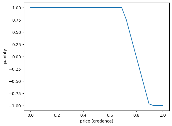
As you can see, this trading formula says to purchase 1 token of sentence1 whenever that sentence's price, or credence, is below 0.8, or zero tokens if the price is above 0.8. Actually there is a region just around 0.8 where the quantity move linearly from 1 down to 0 -- this is actually very important.

Now we define a trading algorithm

A trading algorithm is a generator of trading policies, which are maps from sentences to trading formulas

def trading_alg(sentence, probability):
    count = 1
    while True:
        yield {sentence: trade_on_probability(sentence, count, probability)}
        count += 1

Create a logical inductor and perform two updates

inductor = li.LogicalInductor()

first_credences = inductor.update(sentence3, trading_alg(sentence3, .5))

print("after first update:")
for sentence, credence in first_credences.items():
    print(f'  credence for "{sentence}"" is {credence}')
    
second_credences = inductor.update(sentence2, trading_alg(sentence3, .5))

print("after second update:")
for sentence, credence in second_credences.items():
    print(f'  credence for "{sentence}"" is {credence}')

third_credences = inductor.update(sentence1, trading_alg(sentence3, .5))

print("after third update:")
for sentence, credence in third_credences.items():
    print(f'  credence for "{sentence}"" is {credence}')

    after first update:
      credence for "socrates is a man"" is 0
      credence for "socrates is a man → socrates is mortal"" is 0
    after second update:
      credence for "socrates is a man"" is 0
      credence for "socrates is a man → socrates is mortal"" is 1
    after third update:
      credence for "socrates is a man"" is 0
      credence for "socrates is a man → socrates is mortal"" is 1

That's it! The rest of this notebook will explore the inner workings of the update function used above.

Let's look at the inner workings of the logical induction algorithm

First we will get a concrete trading algorithm and pull out the trading policy it uses on the first update.

the_trading_alg = trading_alg(sentence1, .8)

first_trading_policy = next(the_trading_alg)

Now we solve for our a belief state where this trading policty makes very few trades

We are going to find a set of credences that are not exploited by first_trading_policy. The logic for solving for credences is implemented in the library function li.find_credences. For this example will use an empty belief history, just as if this was our very first update ever.

history = li.History()   # empty history
credences = li.find_credences(first_trading_policy, history, tolerance=.01)
credences

    {socrates is a man: Fraction(4, 5)}

We just solved for our first belief state. This belief state contains only one sentence because our trading policy first_trading_policy only trades on one sentence. We can check the quantity traded by our trading policy on the belief state we found:

updated_history = history.with_next_update(credences)
quantity = first_trading_policy[sentence1].evaluate(updated_history)
print('quantity traded is', quantity)

    quantity traded is 0.0

In this case our trading policy traded exactly zero, but any quantity less than the tolerance passed to find_credences would have been acceptable.

Plot the space over which find_credences searches

To get some insight into how li.find_credences works, let us plot the landscape over which it searches. It is looking for a belief state such that the maximum value-of-holdings for the given trading policy is close to zero.

def value_of_holdings_landscape(trading_policy, credence_history, x_sentence, y_sentence):
    min_possible = np.zeros((20, 20))
    max_possible = np.zeros((20, 20))
    for i, x in enumerate(np.linspace(0, 1, 20)):
        for j, y in enumerate(np.linspace(0, 1, 20)):
            credences = {x_sentence: x, y_sentence: y}
            history = credence_history.with_next_update(credences)

            # check all possible worlds (all possible truth values for the support sentences)
            possible_values = []
            for truth_values in itertools.product([0, 1], repeat=2):
                world = {sentence1: truth_values[0], sentence2: truth_values[1]}
                value_of_holdings = li.evaluate(trading_policy, history, world)
                possible_values.append(value_of_holdings)
                
            min_possible[j,i] = min(possible_values)
            max_possible[j,i] = max(possible_values)

    return min_possible, max_possible

_, max_landscape = value_of_holdings_landscape(first_trading_policy, history, sentence1, sentence2)

plt.imshow(max_landscape, extent=(0, 1, 0, 1), vmin=0, vmax=1)
plt.xlabel(sentence1)
plt.ylabel(sentence2)
plt.colorbar()
plt.show()

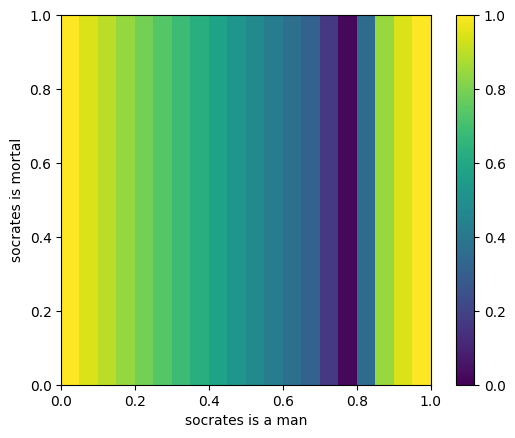
So we can see that this function has a local minimum when the credences for "socrates is a man" is 0.8, and as expected this function does not depend at all on the credence for "socrates is mortal"

Compute a budget factor

To demonstrate the inner workings of the logical induction algorithm, let's look at the structure of a budget factor. Here is the formula from our one-sentence trading policy as a syntax tree:

print(first_trading_policy[sentence1].tree())

    Min
    . Constant(1)
    . Max
    . . Constant(-1)
    . . Sum
    . . . Constant(8.0)
    . . . Product
    . . . . Constant(-10)
    . . . . Price(socrates is a man, 1)

Now let's compute a budget factor and print it as a syntax tree.

budget_factor = li.compute_budget_factor(
    budget=2,
    observation_history=[],
    next_observation=sentence1,
    trading_history=[],
    next_trading_formulas=first_trading_policy,
    credence_history=history)

print(budget_factor.tree())

    SafeReciprocal
    . Max
    . . Product
    . . . Constant(0.5)
    . . . Product
    . . . . Constant(-1)
    . . . . Sum
    . . . . . Product
    . . . . . . Min
    . . . . . . . Constant(1)
    . . . . . . . Max
    . . . . . . . . Constant(-1)
    . . . . . . . . Sum
    . . . . . . . . . Constant(8.0)
    . . . . . . . . . Product
    . . . . . . . . . . Constant(-10)
    . . . . . . . . . . Price(socrates is a man, 1)
    . . . . . . Sum
    . . . . . . . Constant(1.0)
    . . . . . . . Product
    . . . . . . . . Constant(-1)
    . . . . . . . . Price(socrates is a man, 1)

---

1. Really what we get is the guarantee that updates are computable and that therefore at least one algorithm exists. In fact there are many possible concrete algorithms for performing updates in logical induction. ↩︎

8 comments

Comments sorted by top scores.