Beyond Kolmogorov and Shannon

post by Alexander Gietelink Oldenziel (alexander-gietelink-oldenziel), Adam Shai (adam-shai) · 2022-10-25T15:13:56.484Z · LW · GW · 17 comments

Contents

  Compression is the path to understanding
  Standard measures of information theory do not work
    Kolmogorov Complexity
    Shannon Entropy
  Summary
None
17 comments

This post is the first in a sequence that will describe James Crutchfield's Computational Mechanics framework. We feel this is one of the most theoretically sound and promising approaches towards understanding Transformers in particular and interpretability more generally. As a heads up:  Crutchfield's framework will take many posts to fully go through, but even if you don't make it all the way through there are still many deep insights we hope you will pick up along the way.

EDIT: since there was some confusion about this in the comments: These initial posts are supposed to be an introductionary and won't get into the actually novel aspects of Crutchfield's framework yet. It's also not a dunk on existing information- theoretic measures - rather an ode!

To better understand the capability and limitations of large language models it is crucial to understand the inherent structure and uncertainty ('entropy') of language data. It is natural to quantify this structure with complexity measures. We can then compare the performance of transformers to the theoretically optimal limits achieved by minimal circuits.^[1] This will be key to interpreting transformers. 

​The two most well-known complexity measures are the Shannon entropy and the Kolmogorov complexity. We will describe why these measures are not sufficient to understand the inherent structure of language. This will serve as a motivation for more sophisticated complexity measures that better probe the intrinsic structure of language data. We will describe these new complexity measures in subsequent posts. Later in this sequence we will discuss some directions for transformer interpretability work.

Compression is the path to understanding

Imagine you are an agent coming across some natural system. You stick an appendage into the system, effectively measuring its states. You measure for a million timepoints and get mysterious data that looks like this:

...00110100100100110110110100110100100100110110110100100110110100...

You want to gain an understanding of how this system generates this data, so that you can predict its output, so you can take advantage of the system to your own ends, and because gaining understanding is an intrinsic joy. In reality the data was generated in the following way:  output 0, then 1, then you flip a fair coin, and then repeat. Is there some kind of framework or algorithm where we can reliably come to this understanding?

As others have noted, understanding is related to abstraction [LW · GW], prediction [LW · GW], and compression [LW · GW]. We operationalize understanding by saying an agent has an understanding of a dataset if it possesses a compressed generative model: i.e. a program that is able to generate samples that (approximately) simulate the hidden structure, both deterministic and random, in the data.​^[2] 

Note that pure prediction is not understanding. As a simple example take the case of predicting the outcomes of 100 fair coin tosses. Predicting tails every flip will give you maximum expected predictive accuracy (50%), but it is not the correct generative model for the data. Over the course of this sequence, we will come to formally understand why this is the case.^[3]

Standard measures of information theory do not work

To start let's consider the Kolmogorov Complexity and Shannon Entropy as measures of compression, and see why they don't quite work for what we want.

Kolmogorov Complexity

Recall that the Kolmogorov(-Chaitin-Solomonoff) complexity $K\left(x\right)$ of a bit string $x$ is defined as the length of the shortest programme outputting $x$ [given a blank output on a chosen universal Turing machine]

One often discussed downside of the K complexity is that it is incomputable. But there is another more conceptual downside if we want Kolmogorov complexity to measure structure in natural systems: it assigns maximal 'complexity' to random strings.  

Consider again the 0-1-random sequence 

...00110100100100110110110100110100100100110110110100100110110100...

The Turing Machine is forced to explicitly represent every randomly generated bit, since there is no compression available for a string generated by a fair coin. For those bits, we will have to use up a full 1 bit (in this case 10E6/3 bits total). For the deterministic 0 and1 bits, we need only remember where in the sequence we are: the deterministic 0 position, the deterministic 1 position, or the random position. This requires log(3) ~= 1.58 bits. 

There are two main things to note here. First, the K complexity is separable into two components, one corresponding to randomness, and the other corresponding to deterministic structure. Second, the component corresponding to randomness is a much larger contributor to the K complexity, by 6 orders of magnitude! This arises from the fact that we want the Turing Machine to recreate the string exactly, accounting for every bit.

If we want to have a compressed understanding of this string, why should we memorize every single random bit? The best thing to do would be to recognize that the random bits are random, and simply characterize them by the entropy associated with that token, instead of trying to account for every sample. In other words, the program associated with the standard way of thinking of K complexity is something like:

# use up a lot of computational resources storing every single
# random bit explicitly. This is a list that is 10E6/3 long!!!
random_bits = [0, 1, 1, 1, 1, 0, 0, 1, 
				...,
				...,
				...,
				0, 0, 1, 1, 0, 1, 0, 0]

# a relatively compact for-loop of 3 lines. the last line fetches the stored
# random data
for i in range(data_length/3):
	data.append(0)
	data.append(1)
	data.append(random_bits[i])

The first line of code memorizes every random bit we have to explicitly represent. Then we can loop through the deterministic 0-1 and deterministically append the "random" bits one by one. But here's a much more compact understanding:

for i in range(data_length/3):
	data.append(0)
	data.append(1)
	data.append(np.random.choice([0,1])

Note that the last line of this program is not the same as the last line of the previous program. Here we loop through appending the deterministic 0-1 and then randomly generate a bit. 

If we were right in our assessment that the random part was really random then the first programme will overfit: if we do the observation again the nondeterministic part will be different - we've just 'wasted' ~${10}^6$ of bits on overfitting! 

The issue with K complexity is that it must account for all randomly generated data exactly. But an agent trying to create a compact understanding of the world only suffers when they try to account for random bits as if they were not random. A Turing Machine has no mechanism to instantiate uncertainty in the string generating process.

Shannon Entropy

Since K complexity algorithmically accounts for every bit, whether generated by random or deterministic means, it overestimates the complexity of data generated by an at least partially random processes. Maybe then we can try Shannon Entropy since that seems to be a measure of the random nature of a system. As a reminder, here is the mystery string:

...00110100100100110110110100110100100100110110110100100110110100...

Recall that the Shannon Entropy of a distribution $p\left(x\right)$ is $-{\sum }_{x}p\left(x\right)log\left(p\right(x\left)\right)$, and that entropy is maximized by uniform distributions, where randomness is maximum. What is the Shannon Entropy of our data? We need to look at the distribution of 0s in 1s in our string:

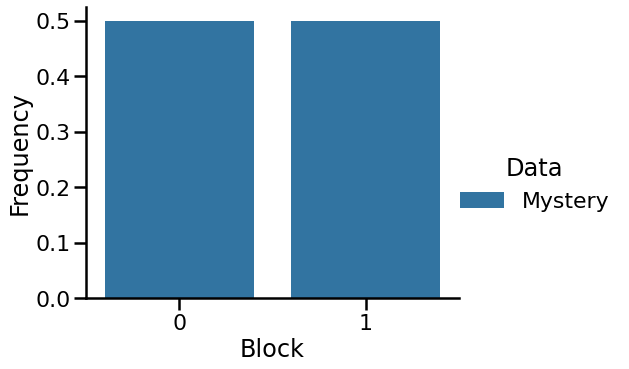
There are equal numbers of 0's and 1's in our data, so the Shannon Entropy is maximized. From the perspective of Shannon Entropy, our data is indistinguishable from IID fair coin flips! This corresponds to something like the following program:

for i in range(data_length):
	data.append(np.random.choice([0,1])

which is indeed very compact. But it also does not have great predictive power. There is structure in the data which we can't see from the perspective of Shannon Entropy. Whereas the perspective of K complexity led to overfitting the data by treating randomly generated bits as if they were deterministically generated, the perspective of Shannon Entropy is akin to under fitting the data by treating deterministic structure in the data as if it were generated by a random process.

Summary

These are the key takeaways:

• Data is, in general, a mixture of randomly generated components and deterministic hidden structure
• We understand understanding as producing accurate generative models. 
• Kolmogorov Complexity and Shannon Entropy are misleading measures of structure. Kolmogorov complexity overestimates deterministic structure while the Shannon Entropy rate underestimates deterministic structure.
• We need a framework that allows us to find and characterize both structured and random parts of our data.

As a teaser, the first step in attacking this last question will be investigating how the entropy (irreducible probabilistic uncertainty) changes at different scales. 

 

1. ^{^}

   In Crutchfield's framework these are called 'Epsilon Machines'. 

2. ^{^}

   Understanding is not just prediction - since prediction is a purely correlational understanding that does in general lift to the full causal picture. Recall that for most large data sets there are many causal models compatible with the empirical joint distribution. To distinguish these causal models we need interventional data. To have 'deep' understanding we need full causal understanding. 

3. ^{^}

   A simple way to see that All Tails is not the correct generative model is to consider sampling it many times: the observed empirical distribution of sampling from Tailx100 is very different from CoinFlipx100

17 comments

Comments sorted by top scores.