An introduction to language model interpretability
post by Alexandre Variengien (alexandre-variengien) · 2023-04-20T22:22:49.519Z · LW · GW · 0 commentsContents
  Introduction
  Two Whys
    A toy model of target features for self-supervised models
    Caveats of the toy model
    Sidenote: The anthropomorphization bias
  Two Hows
  Choosing a task
  Interpreting the model
  Communicating results
None
No comments
This document was written while working at Redwood Research as part of the training material for REMIX. Its goal was to introduce useful considerations before beginning empirical work on language model interpretability. It assumes familiarity with causal scrubbing [LW · GW], and the work on IOI.
While it's technically already publicly accessible from the REMIX github repo, I repost it here with minor edits to make it more visible, as it could be helpful for newcomers to the field of LM interpretability.
Introduction
So you have a language model, and you want to do interp to explain how it implements a particular behavior. Or maybe you're still searching for a behavior to explain. Before jumping straight into defining a task or running experiments, it is useful to contextualize your subject of study. How to think about language model behaviors? How are they shaped by the training process? For a given model behavior, what structure in the model internals should I expect to find?
These are hard questions, and we are far from having definitive answers to them. Here, I'll present a toy model enabling informed guesses in practical cases. It's better seen as a "scaffolded intuition" than a proper theoretical framework. After introducing the toy model, I'll end with a list of practical advice for LM interp research.
To start the reasoning, I found it useful to borrow questions from ethology. After all, this is another field studying behaviors in organisms selected for maximizing a particular objective (fitness) function. I’ll go through an adaptation of Tinbergen's four questions — two “why” and two “how” — to think about what are “behaviors”.
Two Whys
Why #1 - Function - Why does the model learn this behavior on this input distribution rather than something else? How does the behavior affect the model loss on its training set?
In the case of language models, what are the features present in text data that the behavior is mimicking? In other words: If a language model is a butterfly that mimics the appearance of leaves, what is the exact shape of the leaf's veins it’s trying to imitate?

If you don’t have any convincing story for the previous question, maybe it’s because the behavior you're looking at is not a useful mechanism to model training data. It can be the side effect of a useful mechanism. For instance, text-ada-001 completes the prompt “This&is&a&sentence&” by a loop of “&is&a&sentence&” separated by a skipped line. I’m not sure that this particular behavior corresponds to any meaningful feature of internet text data. It's likely that the prompt is far out of distribution, that the model is in “high uncertainty mode”, and so it uses basic heuristics that are generally useful, like repeating text.
In all cases, it’s important to differentiate between the target feature the behavior is mimicking, and its approximation implemented by the behavior (which is often hard to fully characterize). E.g. on IOI, the feature is “identify a plausible indirect object from the context”, and the behavior implemented by GPT2-small is roughly “look for non-duplicated names in the context”. The two functions overlap enough that this is a good strategy to minimize the loss in training.
A toy model of target features for self-supervised models
The goal of self-supervised language models is to predict a next-token probability distribution that imitates the large pile of text they saw in training.
As a simplified model, we can think of the training distribution as a set of target features to imitate.[1] Some of those features are “The name used as an indirect object appeared previously in the context”, “When a sentence is ending in a quotation mark, a closing quotation mark follows”, “After ‘Barack’ often comes ‘Obama’” etc. Each target feature is a task to solve for the language model.
In this model, target features are disjoint such that the total loss on the training set is the sum of the losses on each individual target feature, weighted by how frequently they appear in the training set.
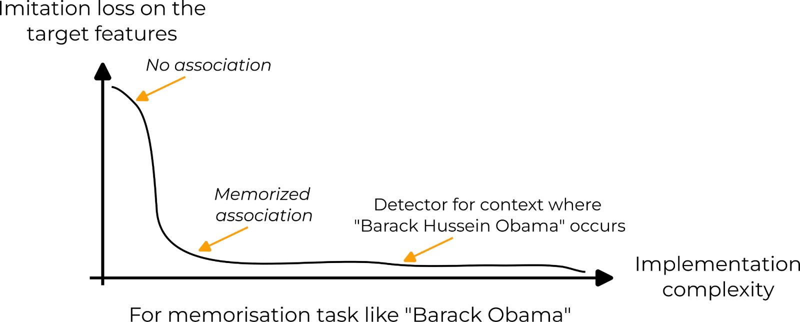
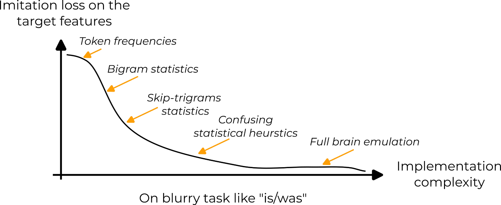
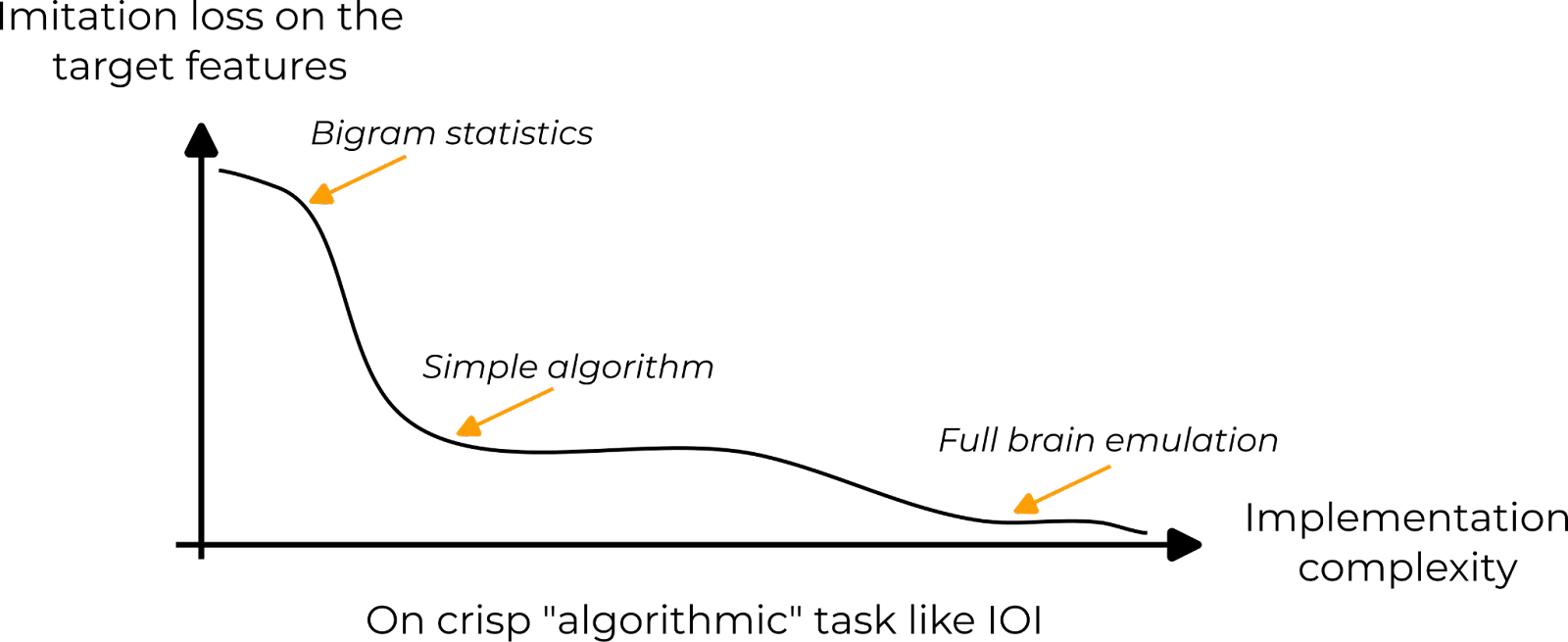
If we zoom in on a particular target feature, we can ask: given a model and a limited implementation capacity, what is the best approximation of the target feature I can find? In other words: what is the Pareto frontier of the imitation loss and complexity budget? Each point on this line is a behavior mimicking the target features.
Depending on the task, this graph will look different. For instance, on a memorization task like predicting “Obama” after “Barack”, the shape is a sharp transition from no association to a learned association. More advanced tricks can be learned with sufficient complexity budgets. For instance, detecting contexts where Obama’s full name (Barack Hussein Obama II) will be used instead of the short version. But such fancy tricks require a lot of model capacity while only making little gain in imitation loss.
Some target features require understanding subtle clues in the sentence, e.g. choosing if the next token should be “is” or “was”. It is hard to describe exactly how such features could be implemented with a Python program. They often rely on fuzzy concepts like “the likely tense of a sentence”, “the sentiment of the sentence” etc. To imitate these features, there is a sequence of increasingly complex statistical heuristics. Simple models could use bigrams statistics while on the (unrealistic) very far end of the complexity spectrum, models could simulate human brains to extract statistics about how humans tend to complete such sequences.
Finally, other target features are in between the two previous types. There exists a simple algorithm that is much better than memorized statistics, e.g. because the next token can be retrieved from the context, as in IOI.
After shaping the landscape of the target feature approximation, we need to discuss what pushes a model to choose a particular tradeoff, a particular point on the curve.
We can see a language model as a reservoir of complexity. During training, its job is to
- Allocate its complexity budget to target features according to their importance.
- For each target feature, optimize its approximation given the allocated budget.
As the loss is averaged over the training dataset, the importance of target features is their frequency in the training data.
This tradeoff is better illustrated by considering different models. This leads us to the second question.
Why #2 - Comparative Model Analysis - Why does this behavior exist in a particular model? What is the corresponding behavior in related models (larger / smaller, slightly different architectures), and what are the architecture details necessary for it to arise?
By changing the model, you change
- The total complexity budget. Bigger models trained for longer, have more complexity, and thus can better approximate more target features.
- The meaning of the “implementation complexity” axis is in the above graphs. Different architectures have different inductive biases, making some heuristics harder/easier to implement.
It’s important to keep track of those two points when considering a model: “Does this model have enough capacity to store excerpts from Hamlet?”, “In a Transformer architecture, is the algorithm for 2-digit addition more complex than a lookup table?” etc.
Caveats of the toy model
We cannot consider target features in isolation. In reality, the behavior implementations are all running in parallel and interacting. However, the toy model can be good enough in practice. LM seems to have a strong gating mechanism that allows certain behavior to be expressed and not others (e.g. the French-speaking part of the LM doesn’t fire in the middle of an English text).
But there are cases where the interaction cannot be ignored. Take the example of an important target feature, F, which is modeled by behavior B. There can be a target feature G that is less important but resemble F. On G, the LM will execute B, despite not being a good approximation of the feature G.
Generally, this toy model rests on many ill-defined quantities such as implementation complexity and complexity budget. It is intended as an intuition pump to make you think about useful considerations more than a definitive model of LM behaviors.
Sidenote: The anthropomorphization bias
It’s sometimes hard to make the difference between the model’s behavior and the target features it’s approximating. As humans, it’s easy to project the way we do when we see human-like behavior. General advice applies here: try thinking like an LM and prefer simpler explanations when available.
Two Hows
How #1 - Development - How does the behavior evolve during training? Is there some path dependence in the emergence of the behavior? What training data are necessary for the trained model to display the behavior?
Until now, we considered models performing perfect allocation of their capacity according to the importance of target features, and perfect approximation under those constraints.
In reality, those tradeoffs and approximations are made by a gradient descent-based optimization and are likely to be imperfect. Hence, it's important to keep in mind the specificity of the training process of your model to anticipate deviation from the perfect allocation described above. For instance, if a model is trained with dropout, it is likely that you’ll find component redundancy on the internals, despite not being required to implement the behavior.
How #2 - Causation - How is the behavior implemented in the model’s internals? What are the text features of the prompt that elicit the response?
Finally, this is the question we want to answer by doing interp! I'll not go through a comprehensive description of how to tackle it. Instead, I'll give some advice about various steps along the research process. Some are high-level while some are technical points. Feel free to skip points if they feel too in the weeds.
Choosing a task
With the toy model in mind, here is a set of points to consider when choosing a behavior to investigate.
- What is the importance of the feature in the training data?
- A good way to know which features are important is to play the next-token prediction game.
- What is the shape of the complexity/loss curve on this feature?
- In general, it’s impossible to get. But it’s helpful to make guesses at possible heuristics the model could implement under different budgets.
- Given the size of the model, its inductive bias, and the importance of the feature, where is the behavior placed on the curve?
- This is the crucial question. Ideally, you want a curve that includes a spot with a “simple algorithm” (see the third graph above) and the feature importance/model size/inductive bias are pushing the model on this part of the curve.
- A simple algorithm is much easier to read from the model internals than a pile of statistical heuristics.
Once you have an idea of a task, before answering how the behavior is implemented, it’s helpful to spend some time testing the extent of the behavior, i.e. trying to answer the second causation question.
Interpreting the model
I’ll focus on the step where you have the structure of the circuit (e.g. obtained by path patching) and you try to get a human understanding of what each part is doing. A component refers to an MLP layer or an attention head acting at a particular token position.
- Track the information contained in each part. What is the minimal information that a part can have while still maintaining the behavior? The classical way to answer this question empirically is through causal scrubbing.
- You will not measure what you think you measure [LW · GW]. To limit this, maximize the number of bits your experiments are returning. E.g. when running causal scrubbing, it’s useful to compute several metrics, plot distribution summaries, etc.
- Interp is as much about understanding the model as it is about understanding the dataset. A huge part of the work is about finding the feature that each part is sensitive to (analog to the receptive field).
- The example of S-Inihbition heads in the IOI project. We knew that Name Movers’ used their output to find the indirect object in the context, but we had no idea what information the S-Inihbition heads gave to the Name Movers. In our dataset, there were many ways to do this. S-Inhibition heads could say:
- “Look at the previous occurrence of the token ‘Bob’ ”
- “Look at position 11”
- “Look 5 tokens back”
- “Look at the second token in the context that is a name”
- The goal is then to construct variations of the dataset where those features are decorrelated, perform (path) patching, and observe if the behavior is preserved. (See Appendix A of the paper for more)
- The example of S-Inihbition heads in the IOI project. We knew that Name Movers’ used their output to find the indirect object in the context, but we had no idea what information the S-Inihbition heads gave to the Name Movers. In our dataset, there were many ways to do this. S-Inhibition heads could say:
- In addition, to find what preserves the behavior, it’s helpful to think about the circuit in terms of moving pieces. Imagine a model generating Python code. You identified a component that tracks variable types and sends this information to the latter part of the model. You could try to run this component C on a sequence where the variable
xis an integer while the rest of the model sees a sequence wherexis a boolean. If the model is generating something likeassert type(x) == intthat's a really good sign that C is doing what you think. You used your knowledge about the model's internals to predict how it would behave out of distribution. I found this type of experiment a complementary validation to causal scrubbing that strives to preserve internal distribution under a given hypothesis.
Communicating results
By doing interp, you’ll develop intuition about the roles of each node by ingurgitating a huge number of numerical values. Sometimes it’s hard to put into words why you think what you’re thinking. You’ll spend most of the time confused with half-baked models. A big part of the work is to introspect what are the hidden assumptions you’re making, and what evidence supports those hypotheses, and be ready to update. A good way to do this is to communicate with others.
- Create a first story about how the behavior is implemented. Even if that’s a super simplified view of your fuzzy intuition, it’s a helpful way to put together what you know so far. I would recommend trying to build it quite early on. Lean on the side of claiming stories that are too precise rather than too general, it’s much easier to make progress when you can be proven wrong.
- Create a second story about how you discovered the behavior implementation. Again, it’ll surely not include all the evidence you have. It must be a minimal succession of experiments that rule out concurrent hypotheses to the one you’re claiming. Ideally, each step should be of the form “We knew X and Y, but we didn’t know how Z worked. We had A and B hypotheses for Z, and so we ran experiment E to differentiate between the two”.
- Be clear about what metric you're using, and give extreme examples (what is 0% what is 100%) to explain what is measured and what it’s not.
- Print the standard deviation of your metric when it’s easy to do so and when it’s likely that you’re at the edge of the signal-to-noise ratio.
- When explaining figures, take the time to explain what your interlocutor is seeing, e.g. by taking a particular point as an example. Emphasize what's surprising.
- Name everything you want to communicate more than 3 times.
- Name the important positions in your sequences.
- Name the component you find. Put the same name on components with the same function and the same mechanism.
- Bad names are better than no names. Putting names on things is useful because it reduces cognitive load by grouping components instead of reasoning about them individually.
- ^
This view is similar to the quantization of model abilities introduced in a recent work (published after the original version of this document).
0 comments
Comments sorted by top scores.


