Towards Understanding the Representation of Belief State Geometry in Transformers
post by Karthik Viswanathan (vkarthik095) · 2025-04-18T12:39:01.251Z · LW · GW · 0 commentsContents
  Mess3 Process 101
    Sequence Generation
    Belief Updates
    Next Token Prediction Loss
  Training a Transformer on Mess3 Sequences
  Beyond Stochastic Parrots: Do Transformers Internalize Beliefs?
    Relating final layer activations and next token predictions
    Relating next token predictions and belief states
    Can we generalize the above statements to other processes?
  Conclusion
None
No comments
Recently, I’ve been trying to understand whether we can extract human-interpretable information from the geometry of internal representations in transformer models. In other words, can we combine ideas from conceptual interpretability (what high-level abstractions a model might be using) with mechanistic interpretability (how those abstractions are implemented in the model’s internals)?
This curiosity led me to the work Transformers Represent Belief State Geometry in Their Residual Stream, [LW · GW] which makes an interesting observation: the geometry of the residual stream closely mirrors, and may even fully capture, the underlying data-generating process. This blog post is my attempt to log my thought process[1] as I work through the related paper arXiv:2405.15943. If you are relatively new to this topic and curious to explore it from the ground up, you’re in the right place, and if not, I hope you’ll still find the walkthrough and commentary a useful companion to the original paper.
The core claim is pretty amazing: that transformers learn to represent probabilistic belief states in the residual stream, even when their underlying structure is fractal. In other words, the transformer models aren't merely stochastic parrots: they are building an internal model of the world, at least in controlled settings. Furthermore, the idea of grounding internal representations in an abstract, yet well-defined quantity like belief states provides a promising top-down approach to interpretability. It offers a compelling balance between conceptual interpretability (what the model represents) and mechanistic interpretability (how it represents it).
In this work, the authors analyze transformer models trained on next-token prediction, where the input sequences are generated by edge-emitting Hidden Markov Models (HMMs). For the purposes of this discussion, I will focus on a specific instance emphasized in the paper: Mess3, a 3-state edge-emitting HMM defined over a small token vocabulary. The objective is to examine how the structure of Mess3 sequences gives rise to complex belief dynamics, and how these dynamics are reflected in the geometry of a trained transformer model’s internal representations.
Mess3 Process 101
Mess3 is a synthetic process that stands for a 3-state edge-emitting Hidden Markov Model (HMM) that generates sequences over a vocabulary . What makes Mess3 interesting is that, despite its apparent simplicity, it induces a highly structured and even fractal-like geometry in the space of belief states - probability distributions over the hidden states, conditioned on observed tokens. This makes it a particularly valuable testbed: it is both tractable and nontrivial, offering a controlled setting to investigate how transformers learn and represent complex latent structure. Studying how transformers internalize such structure provides valuable insights into their learning dynamics and representational expressivity.
Sequence Generation
Credits: This image can be found in Figure 1 from https://arxiv.org/abs/2502.01954
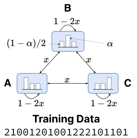
The figure above provides a concise visual summary of the Mess3 process, which helps us understand how sequences are generated. The vocabulary consists of tokens and 3 hidden states . An emission symbol function maps each hidden state to a corresponding token: and . Since this is an edge-emitting HMM, the model emits a token when it transitions from one state to another[2]. As a result, two probabilities govern the generation process: one for transitioning between hidden states, and another for emitting a token conditioned on that transition.
- Transition between hidden states based on the current hidden state which is parameterised with . The transition to the next state given the current state is
The transition probabilities described above can also be inferred from the arrows connecting the states in the figure. Following the setup in the paper, we set . Intuitively, the parameter controls the inertia of a state; lower values of correspond to higher inertia, meaning the system is more likely to remain in the same state across transitions. - Once the next hidden state is chosen, the token emitted is chosen from a probability distribution parameterized by . Given the transition has happened, the probability distribution over the token emitted is given by
Note that the emission probability distribution depends solely on the destination state . This relationship is visually represented by the histograms inside each state in the figure. As in the paper, we set . Intuitively, governs the variability of the emitted tokens: a high value of indicates a strong bias toward emitting the token associated with , the symbol linked to the new state.
So now we have which can be read off from the above expressions. A quantity that will turn out to be useful in the future is the token-labelled transition matrix
Some heuristics in the Mess3 process
We can imagine how tokens are generated now that we are set up.
Let's start at a state = , one likely stays at (with ). Once this happens, it is again highly likely that is emitted (with ). The combined odds of staying at and emitting is , as shown in Figure 1 from this paper.
The odds of moving from to any other state is , and seeing it as a Bernoulli trial, the expected number of turns to move to another state is .[3] If we see the above as a Bernoulli trial, with success as the event of staying at A and emitting 0, i.e. . The expected number of turns for a failure, i.e., seeing another token . Hence, if we are at a state , we can expect the token to repeat thrice.
Here is an example where we show the states and the tokens emitted, where we can approximately see that the states do not change a lot, and the tokens tend to change approximately once every 4 turns.
| States | 1 | 0 | 0 | 1 | 1 | 1 | 1 | 1 | 1 | 1 |
| Tokens | 1 | 0 | 0 | 2 | 1 | 1 | 1 | 1 | 0 | 1 |
Belief Updates
Now that we have a handle on how sequences are generated, let’s turn to the problem of predicting the next token given a sequence of observed tokens (i.e., the context). To model the next token probabilities in Mess3 process, we use a belief state , which represents a probability distribution over the hidden states. The belief state captures our uncertainty about the current hidden state of the Mess3 process, conditioned on the observed token sequence. For a sequence , the belief state represents the probability distribution over the current hidden state, given all observed tokens. That is, , where is the hidden state reached after the transition (i.e., after emitting ).
Since the hidden states are not observed directly, a model trying to predict the next token must maintain a belief state, a probability distribution over which hidden state it's currently in, based on the observed tokens so far. Remarkably, this belief state is all that’s needed to model the process[4]. More precisely, if an observer has seen a sequence and wishes to predict future tokens, they don’t need access to the full sequence history; it suffices to use the current belief state . Mathematically, this amounts to:
When , i.e. before observing any tokens, the belief state is initialized to (the prior) since it corresponds to the stationary distribution in the Mess3 process. Now, suppose we have observed a sequence with tokens and currently maintain a belief state . Upon observing a new emitted token , the question becomes: how should we update our belief state to a new posterior ?
The beliefs are updated using the Bayes' rule: . Since the belief state fully captures the information in the observed sequence , we can replace it with in the above expression which results in:
In matrix notation, we have or , resulting in the belief update equation,
Example of a belief state update
Below we consider the sequence and show how the belief states update after observing each emission.
| Current Belief state | Emission | Updated Belief state | ||||
|---|---|---|---|---|---|---|
| 0.33 | 0.33 | 0.33 | 2 | 0.08 | 0.08 | 0.85 |
| 0.08 | 0.08 | 0.85 | 2 | 0.01 | 0.01 | 0.97 |
| 0.01 | 0.01 | 0.97 | 2 | 0.01 | 0.01 | 0.99 |
| 0.01 | 0.01 | 0.99 | 1 | 0.04 | 0.40 | 0.57 |
| 0.04 | 0.40 | 0.57 | 1 | 0.02 | 0.88 | 0.11 |
| 0.02 | 0.88 | 0.11 | 0 | 0.43 | 0.48 | 0.08 |
| 0.43 | 0.48 | 0.08 | 0 | 0.89 | 0.09 | 0.02 |
| 0.89 | 0.09 | 0.02 | 0 | 0.98 | 0.01 | 0.01 |
| 0.98 | 0.01 | 0.01 | 2 | 0.56 | 0.04 | 0.40 |
| 0.56 | 0.04 | 0.40 | 0 | 0.93 | 0.01 | 0.06 |
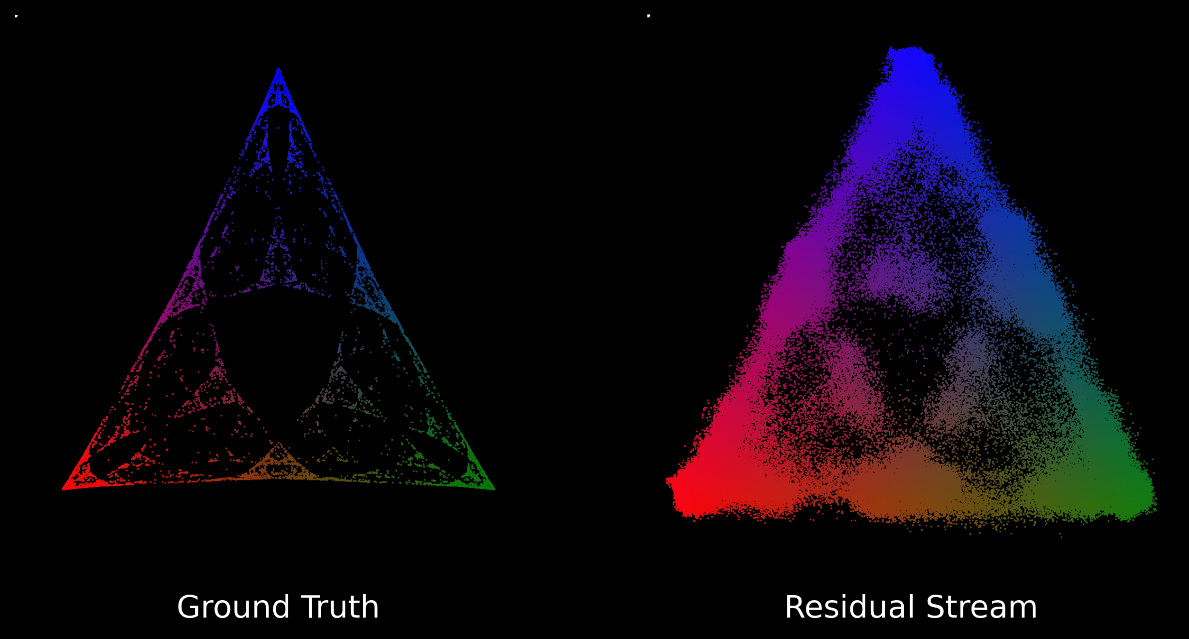
We are going to represent the probability distribution over the belief states as a triangle (since we have ), where each corner corresponds to a hidden state. To summarize, these belief states evolve over time using Bayes' rule, incorporating the latest token and the model's transition-emission structure. The resulting sequence of belief states forms a trajectory through the probability simplex over 3 states (a triangle), and in Mess3, these trajectories form self-similar fractal structures. The fractal structure[5] can be attributed to the recursive nature of the belief update equations, but I hope to find a more detailed explanation for this in the future. For now, we can visualize the sequence of belief states on the 2-simplex that correspond to a long emission.
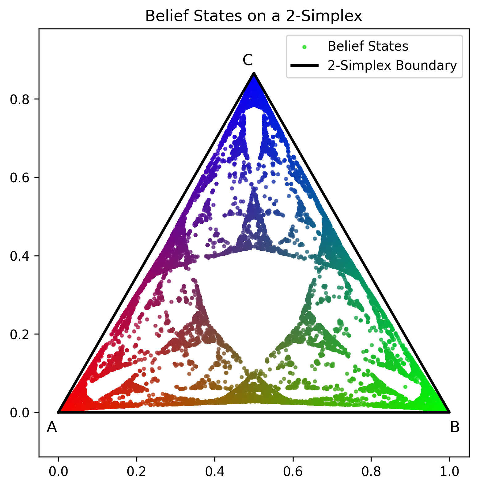
What's pretty cool is that the transformer appears to learn this fractal structure, precisely and linearly, in its residual stream.
Next Token Prediction Loss
We can now use the belief states to perform next token prediction and find the empirical loss for a given prompt. This is a useful exercise since it can inform us as to when the transformer is trained. Given the sequence observed until now and its associated belief state , the next token prediction probability
We can compute this quantity for a batch of sequences and understand the associated empirical loss
The empirical loss over 10000 prompts is around 0.83, and this will be helpful us determine if a transformer is trained on the Mess3 process. This is the best possible average loss achievable by any model, since it is obtained from the ideal model that knows the underlying HMM exactly.
Why do we expect a per-token loss of around 0.83?
Here, we take a prompt with a loss of around 0.86 and track the next token prediction loss for each token in the prompt.
| Current Belief State | Emissions | |
| [0.33, 0.33, 0.33] | 1 | 1.10 |
| [0.08, 0.85, 0.08] | 1 | 0.39 |
| [0.01, 0.97, 0.01] | 0 | 2.10 |
| [0.42, 0.54, 0.04] | 1 | 0.76 |
| [0.07, 0.92, 0.01] | 1 | 0.33 |
| [0.01, 0.98, 0.01] | 1 | 0.27 |
| [0.01, 0.99, 0.01] | 1 | 0.27 |
| [0.01, 0.99, 0.01] | 1 | 0.27 |
| [0.01, 0.99, 0.01] | 0 | 2.14 |
| [0.4, 0.57, 0.03] | 0 | 0.98 |
We can observe from the above table that the per-token loss has a couple of important contributions that are highlighted in bold. It does look like the model is surprised by the emissions at this point. As discussed previously, we can expect these surprises to happen once every 4 turns, which is roughly consistent with the above table.
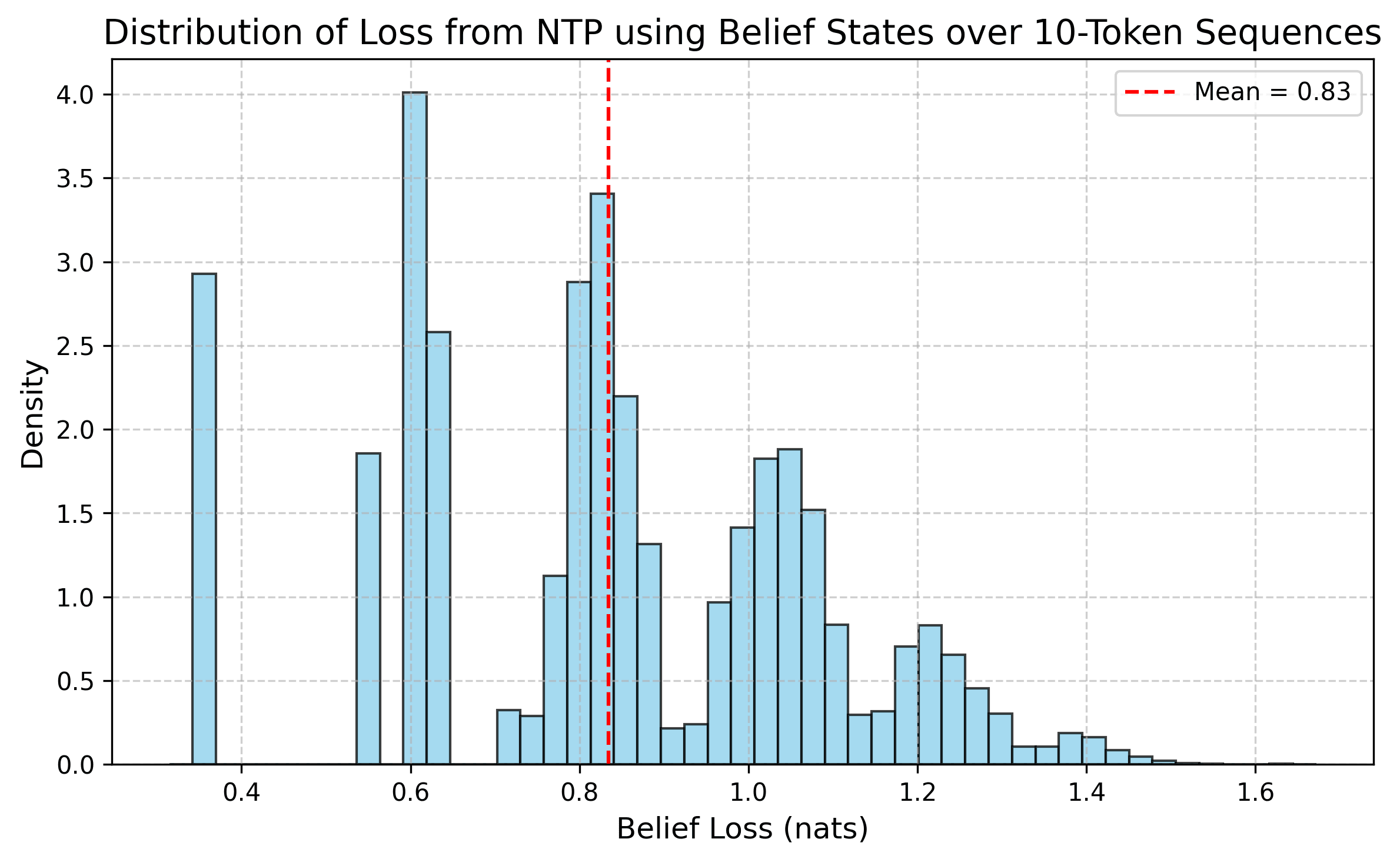
Distribution of Loss using the Belief State Model
In this figure, we visualize the distribution of loss over 10-token sequences to gain an empirical understanding of the variability in prediction quality when using the belief state model. The different peaks in the loss histogram suggest a different physics for the corresponding prompts, which can be interesting to look into.
Training a Transformer on Mess3 Sequences
Now that we’ve explored the Mess3 process, let’s move on to training a transformer model. We'll follow a setup similar to the one described in Appendix A.6 of arXiv:2405.15943. For completeness, I’ve included the relevant hyperparameters below.
Model architecture and training hyperparameters
# --- Model Parameters ---
config = HookedTransformerConfig(
           d_model=64,
           d_head=16,
           n_layers=3,
           n_ctx=100,
           n_heads=4,
           d_mlp=256,
           d_vocab=3,
           device="cuda",
           act_fn="relu",
       )
model = HookedTransformer(config)

# --- Training Parameters ---
optimizer = torch.optim.Adam(model.parameters(), lr=1e-4)
BATCH_SIZE = 128
SEQ_LEN = 10
NUM_EPOCHS = 10001
Transformer loss vs belief state model loss on 1000 prompts
In the plot below, we take prompts, calculate the empirical loss on each prompt from the transformer model and the belief state model, and scatter plot these quantities.
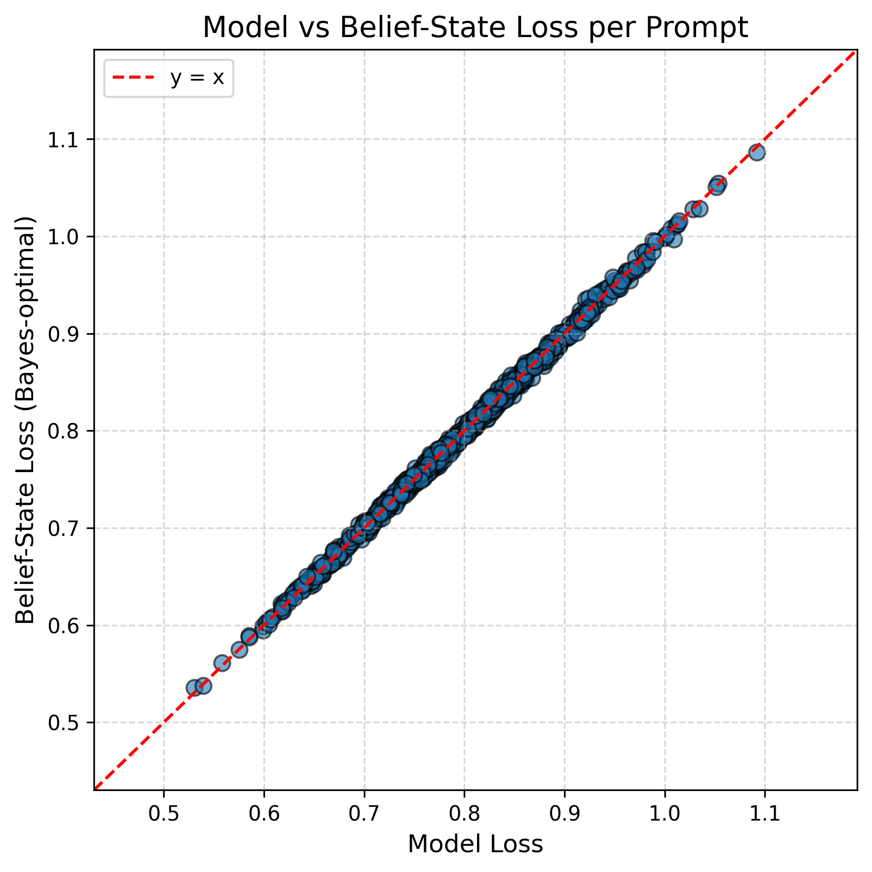
The losses roughly lie on the line which suggests that the model is trained.
We train the transformer with layers and attention heads for epochs on batches of prompts to learn the Mess3 process, which seems to be a bit excessive to predict the probability of the next token in a vocabulary of words. Nevertheless, this results in a neat[6] fractal structure as shown in the figure below.
In fact, we can also see how the fractal structure develops over epochs in the GIF below:
Beyond Stochastic Parrots: Do Transformers Internalize Beliefs?
To sum up, we have seen that the residual stream (specifically the final layer activations) captures a geometry that mirrors the belief states of the Mess3 process. This is striking, given that the transformer has no explicit knowledge of the underlying process. Yet, the same fractal structures that emerge in the belief states also appear in the model’s internal representations.
Although transformers excel as stochastic parrots, must they maintain an accurate model of belief states to do so effectively?
I suspect that the true answer lies within the framework of computational mechanics, and it is far from straightforward. To get some intuition, we simplify the question by focusing on the specific case of the Mess3 process. My hypothesis is that if a model has perfectly learned the Mess3 process, then we should indeed expect a fractal structure to emerge in the final layer activations[7]. This can be understood by studying the geometric relation between
- Final layer activations and the resulting next token predictions
- Next token predictions and the related belief states
Relating final layer activations and next token predictions
The paper Implicit Geometry of Next Token Prediction reports that, in models trained on next-token prediction, contexts that share the same support over possible next tokens tend to produce final layer activations that are close in representation space.
Given final layer activations for a context , the next token prediction can be written as
While we can imagine the unembedding to preserve the geometry of the final layer activations , it remains to be understood if the subsequent softmax operation also preserves this geometric structure. Softmax is invertible up to normalization, and since we are dealing with normalized final layer outputs, this is an invertible operation that can preserve fractal geometry if present.
Relating next token predictions and belief states
The relation between the next token prediction and can be written as
Hence there exists a linear[8] relation between the next token prediction and belief states given by .
How is this linear mapping relevant? Let's say we have the ideal transformer that can find the exact next token prediction probabilities for any given context . If the matrix is bijective, the geometry of the belief states can be similar to the next token prediction probability geometry in the ideal transformer.
In summary, the relation between the final layer activations and the belief states for the Mess3 process can be written as a sequence of operations given below
where is the final layer activations for a context . In words, the above equation is
For Mess3 process when , the unemebedding is a linear operation and the softmax and the multiplication by are invertible. This suggests that we can expect the fractal geometry in the belief states to show up in the final layer activations.
Can we generalize the above statements to other processes?
The short answer is: no, and this is where things become interesting.
The key issue in generalizing is that similar next-token predictions do not always imply proximity in belief space, i.e., the mapping matrix may not be invertible in general. In processes like RRXOR, distinct belief states can give rise to nearly identical next-token distributions. When this happens, the geometry of the belief states becomes compressed in the prediction space, making it impossible to reconstruct belief geometry from activations alone. In such cases, as demonstrated in arXiv:2405.15943, the geometry of the belief states is not fully captured at the final layer alone but is instead distributed across multiple layers of the residual stream. This is a particularly intriguing finding, and one that I hope to explore further in future blog posts.
Conclusion
Through the lens of the Mess3 process, we have seen that transformers are capable of internalizing complex, structured belief states by reflecting their fractal geometry within the residual stream. This challenges the view of transformers as mere "stochastic parrots" and instead supports a richer perspective: that, at least in structured synthetic settings, these models appear to learn compact internal representations that approximate the latent probabilistic processes generating the data.
The analysis suggests that when the mapping from belief states to next-token predictions is invertible, and the transformer is sufficiently trained, the belief geometry can be linearly embedded into the model’s final layer representations. However, this clean correspondence breaks down in other settings like RRXOR, where the prediction space loses information about the underlying beliefs. In such cases, the belief state geometry is not localized to a single layer but is distributed throughout the residual stream, raising exciting questions about the depthwise structure of representation in transformers.
I'm particularly excited to see more work in the spirit of arXiv:2502.01954, where the authors reverse-engineer the role of an attention block. One question that especially interests me is: what happens when we stack multiple attention blocks and layers? Can we gain a more precise understanding of how these components "communicate" and coordinate to implement belief state updates?
Stay tuned, I'll be diving into some of these topics in the next post!
Acknowledgment: This blog post was developed as part of my application to the MATS 8.0 program. It began as an effort to understand one of the recommended references listed on the application page: arXiv:2405.15943.
- ^
This involves clarifying what makes sense to me, highlighting areas of confusion, and exploring how these ideas might connect to larger themes in interpretability and representation learning.
- ^
Note that this includes self-transitions, i.e. moving from a state to itself.
- ^
Perhaps this is the motivation for setting the context length to for the transformer model.
- ^
I find this to be a non-trivial statement for now, perhaps there is a simple explanation related to the definition of HMMs.
- ^
This paper discusses the fractal geometry in HMMs.
- ^
The residual stream projection is not as sharp as I imagined it to be, but I can believe that this can be made sharper given more training time.
- ^
The arguments in the upcoming part are handwavy, but there is scope to make them more formal.
- ^
This bijection holds under certain conditions which includes and .
0 comments
Comments sorted by top scores.