D&D.Sci Hypersphere Analysis Part 4: Fine-tuning and Wrapup

post by aphyer · 2024-01-18T03:06:39.344Z · LW · GW · 5 comments

Contents

  Finetuning our Model
    Latitude
    Shortitude
    Deltitude
    Pi
    Longitude
  Our Final Decision
None
5 comments

As before, this is extreme spoilers for this D&D.Sci scenario [LW · GW], if you want to solve on your own try that first!

 Last time [LW · GW] we got a solution that I'm pretty sure will work.  Everything from here on is just showing off a bit, and seeing if we can find any stuff that abstractapplic didn't expect anyone to get :P.

Finetuning our Model

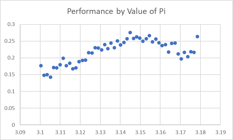
The good news about having a reasonably firm model after last time [LW · GW] is that we now have much better data for looking into any datapoints we want: before our data was extremely noisy, but now that we've controlled out the large majority of variance we're able to zoom in much more precisely on the few remaining effects.  We've gone from having graphs of the effect of Pi that looked like this to vaguely suggest that 'Pi around the true value is probably good':

to having graphs that look like this to highlight that 'we're putting a threshold at 3.14159 when it should be at 3.15':

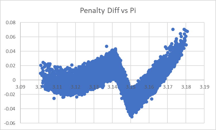
So let's make a pass through all the continuous variables and see if we can get anything else out of them.  We're plotting the value of each variable against the difference between the value of Penalty our model predicts vs. what we actually see: so a positive number means 'our model is predicting a lower penalty, and so higher performance, than actually occurs for sites like this' and a negative number means the reverse.

Latitude

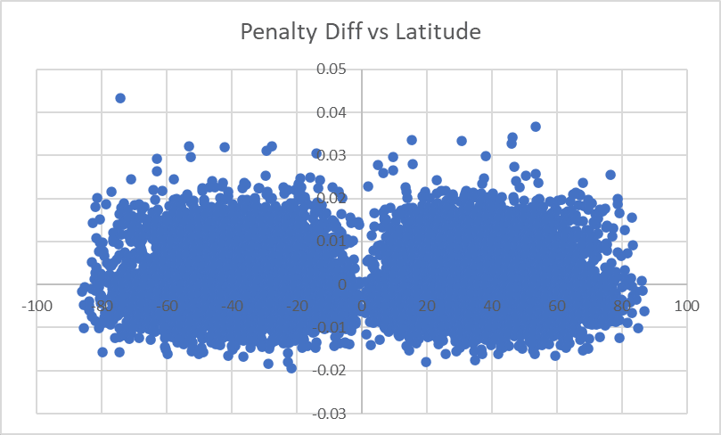
Nothing stands out to fix here.  The two-blobs shape is because latitudes near 0 are rarer.  That single point near the top left is our highest-error site in the universe, hopefully it'll shrink a bit as we fix other things.

Shortitude

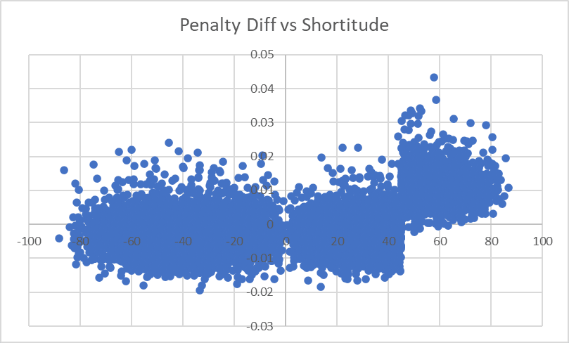
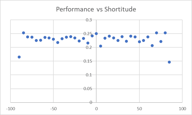
...wow.  Okay, that certainly stands out very dramatically now that we've got a cleaned-up model.  Our initial looks at Shortitude saw things like this:

I guess we just didn't see the effect because it wasn't very big?  A Penalty Factor of...this looks like about 0.015? - corresponds to only a 3-4% drop in performance.  And because of the multiplicative nature of these metrics, a 3-4% drop in average performances around 20-25% would be a <1 percentage point^[1] diff, which we couldn't pick out on that graph but can pick out now.  Let's rerun the model with an extra parameter for [Shortitude is >45]...

...alright, our largest diff has shrunk from 4.74% to 2.72%, that's quite a drastic jump in our confidence.  This doesn't actually change our top-12 list much - not many entries in it had Shortitude>45, and the Shortitude effect is small enough that good sites can remain good even with it - but the fact that our error has shrunk that much means that we're now fairly confident all of our top sites will end up >100%.

Deltitude

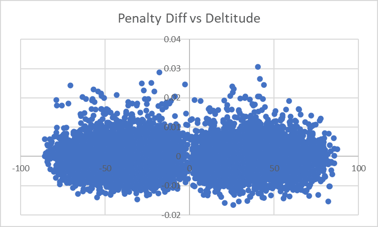
Sadly we don't see any similar effect here.  I'm less certain that there will be one now here now that we've found an effect of Shortitude: the cynical-GM-modeling portion of my brain thinks that one red herring variable is plausible but that two separate ones are very unlikely. 

Pi

Last time, we were including three factors for Pi:

• Low Pi, measuring the amount Pi was below 3.14159 (or 0 if Pi was above that).
• Hi Pi 1, measuring the amount Pi was above 3.14159 (or 0 if Pi was below that).
• Hi Pi 2, measuring the amount Pi was below 3.15 (or 0 if Pi was above that).

These ended up in our most recent model with coefficients of (remember positive=bad, negative=good):

• Low Pi: 5.76
• Hi Pi 1: -4.11
• Hi Pi 2: 8.97

corresponding to a graph of 'what performance penalty do we expect from a given value of Pi' that looks like this:

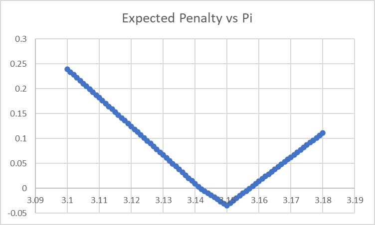
...which yeah, looks very much like we are adding in an additional variable to our model for no good reason.  Let's cut down to 'amount lower than 3.15' and 'amount higher than 3.15', and then look at the factor weights and the residual effect:

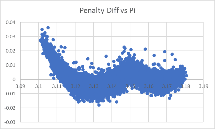
...oooh!  This graph looks like it has a very clear message.  (Stop here and think for a minute if this isn't clear to you and you want to work it out for yourself).

After that change, our largest difference between observed scores and our model is down to 2.08%, and the residual graph for Pi now looks like this:

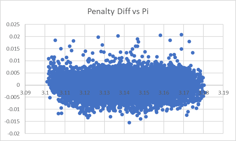
...huh.  This mostly looks right, but on the far left it looks like we actually aren't penalizing the very-far-from-3.15 values of Pi hard enough.  The penalty term grows faster than squared I guess?  If I were doing this seriously I might try to figure out what it was exactly, for now I'll just slap on a difference-cubed term:

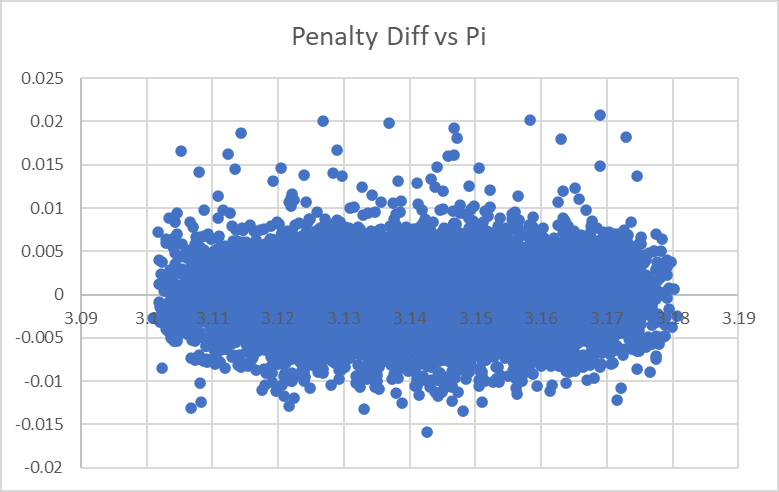
Good enough for government work Our Glorious Empress!

Longitude

Currently we're modeling Longitude's effect as Cosine(Longitude - 50), which looks like this:

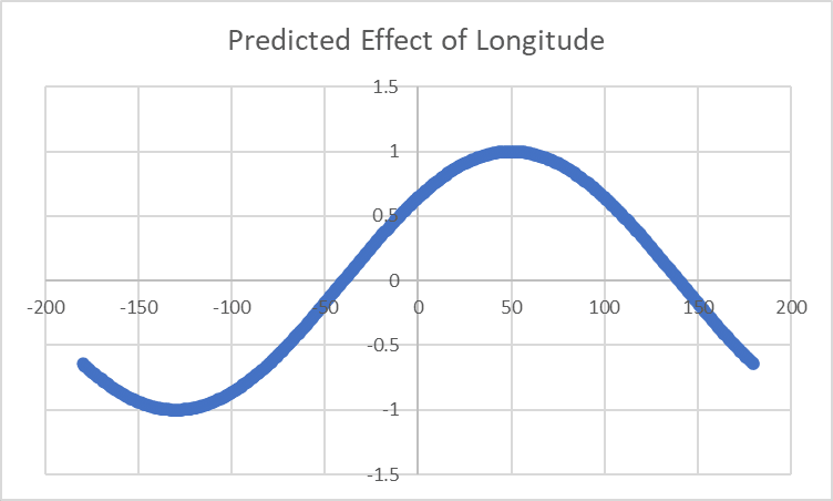
and we're seeing this residual:

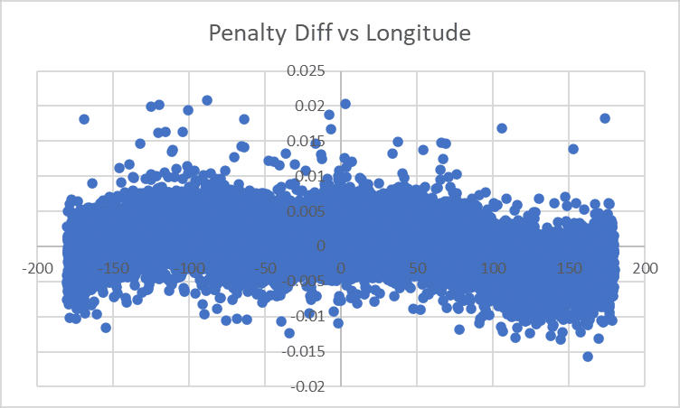
...yeah, this definitely looks like we're not handling Longitude quite correctly, we're overly generous towards things around -100 and overly harsh towards things around +150.

Unfortunately I don't have a good enough head for trig to make ad-hoc adjustments, so let's remove Longitude from the model entirely and see what the effect is when we're just looking at [Effect of Longitude] as opposed to [Effect of Longitude] minus [Our Model's Best Fit To Effect of Longitude]:

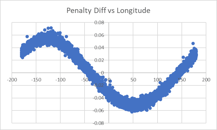
...that really does look like a sine wave bottoming out at exactly 50 degrees.

...after a bit more twiddling, 52 degrees seems to work a bit better, and we have a residual like this:

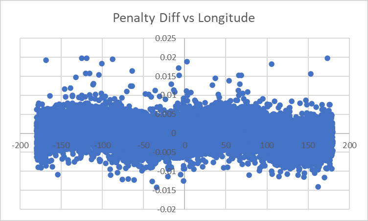
where we can't see as much of a sinusoidal effect, and the largest discrepancy between our model's estimate of performance and the observed value is down to 1.78%.

Murphy's Constant 

Last time, I had no idea how to handle Murphy's Constant, and just flung five different parameters in and let the model sort it out.  The model settled on penalty coefficients of:

• -0.022035 * MC
• -0.024363 * MC^2
• +0.078337 * 2^MC
• -0.010534 * 3^MC
• +0.001125 * 4^MC

for a predicted penalty curve looking like this:

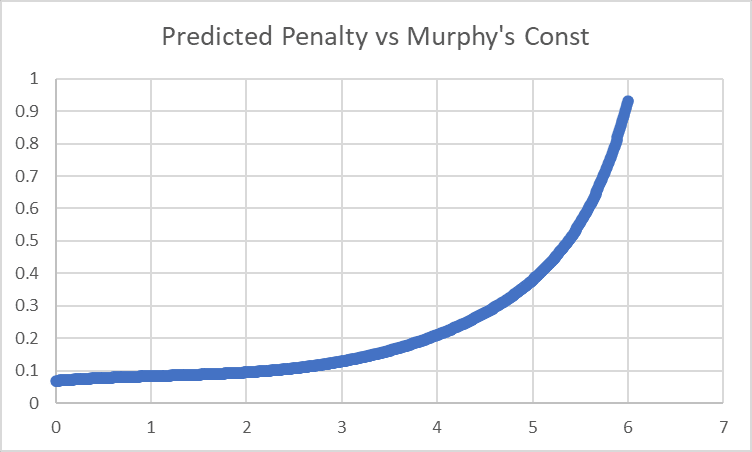
and a residual like this:

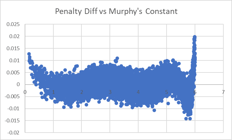
...yeah, that didn't work so great.  Let's try just fitting a degree-6 polynomial to it?

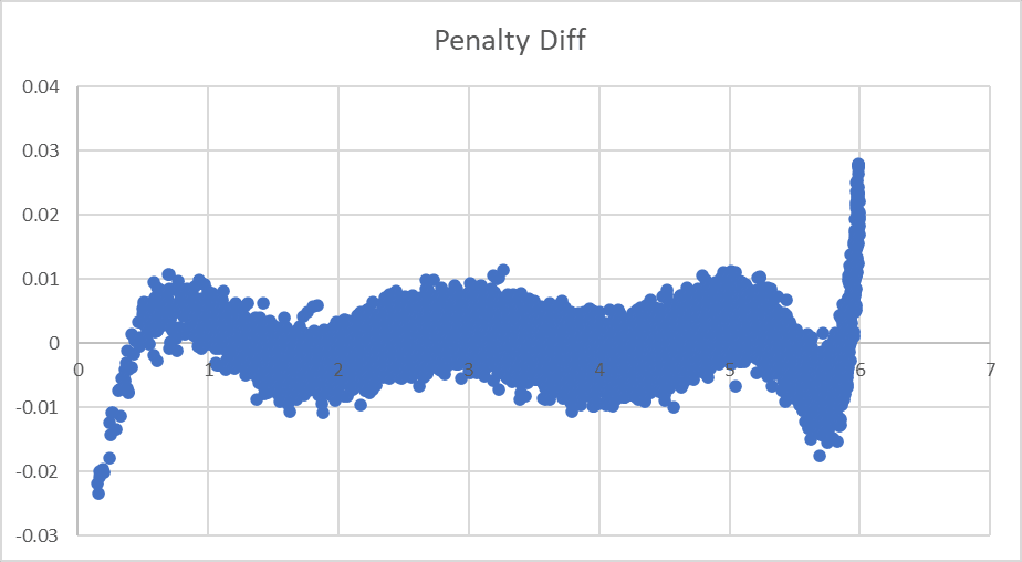
...nnnope.  The abrupt spike at 6 would make me try for a term of 1/(6-MC), except that there are values of MC=6 where that would be infinite.

Let's look at the penalty curve and see what we can fit to it:

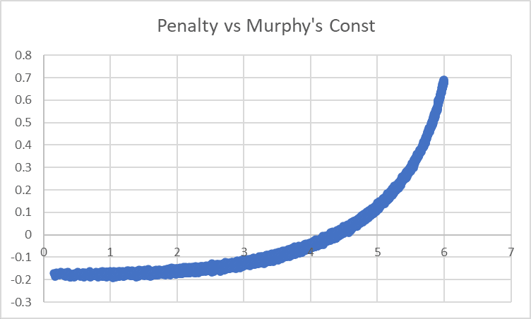
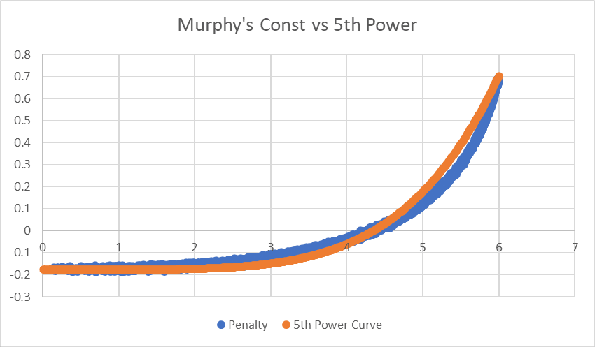
The problem is that it grows very steeply, and with polynomials we need MC^5 to even come close:

What about a 1/(7-MC) term?

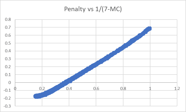
...jackpot!  When we replace our existing Murphy-mess with a term for 1/(7-MC), though, it doesn't quite work:

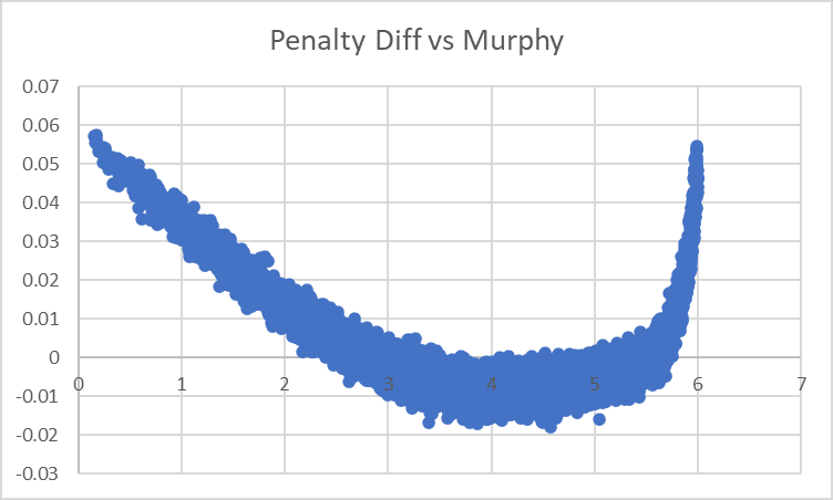
At first I thought we were still missing a term or two.  However, on reflection, it looks like the problem is just that 1/(7-X) is not quite right, and the graph looks approximately straight for various denominators:

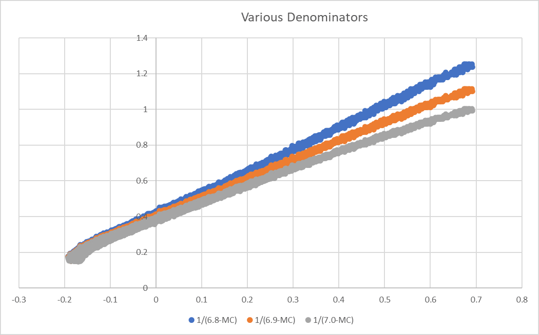
We can try to narrow things down with repeated regressions though.  For example, with a 6.9 in the denominator we see this:

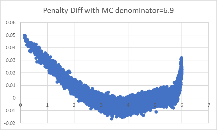
with a spike up on the right indicating that we are being too favorable to values very near 6, and need a smaller denominator.

With a 6.7 in the denominator, we see this:

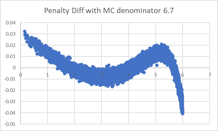
where we're now being too unfavorable to values near 6, and need a larger number in the denominator.

Both show high values on the left side, indicating that the 1/(X-MC) isn't the whole deal (and matching the little bump we see on the left of the original chart).  We could try fitting that with something linear?  But given what we've seen so far maybe we should instead try e.g. a 1/MC or 1/MC+1 term? 

Eventually I lost patience trying to finetune things and just flung a bunch of different variables with slightly different denominators into the regression.  The result seems to have fit very nicely:

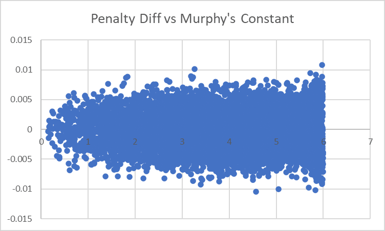
and I'm not really worried about overfitting, since I can see that the graph of penalty vs MC is reasonable.

Still, I think there ought to be a neater way to approach this, and would be very interested if anyone had any ideas for what other residuals are present in the Murphy's Constant effect/how we can predict it with fewer variables.

With this change made, our largest diff is down to 1.44% (not a very large improvement), but we're also more confident in e.g. how the model will perform for very low values of Murphy's Constant (before we were actually systematically overoptimistic about very low values of MC, which was potentially dangerous).

Our Final Decision

With our revised model, we can predict our newest top 12 sites:

Site_ID	Predicted Score
96286	112.6%
9344	110.3%
68204	109.6%
107278	109.4%
905	108.9%
23565	108.3%
8415	106.7%
62718	106.2%
42742	106.0%
83512	105.8%
16423	105.7%
94304	105.2%

This list really hasn't changed very much since last time:

• Site 43792 is the only site from our previous list to no longer be included.  (Its Shortitude of 47.89 degrees puts it just in the Dangerously Short Zone, and it was only midway on our list before). 
• It's been replaced with Site 94304, a marginal new site that just barely didn't make it in last time.
• We're also noticeably less optimistic about Site 23565 than we were before: again it's in the Dangerously Short Zone, and while it looks good enough in other ways that we're still picking it.

However, we are much more confident in this list than we were before.  The largest diff we can see between current examples and our current model is 1.44%, less than a third what it was last time and less than a third what it would need to be for any of these sites to drop below 100%.  Also, we've grown more confident in our handling of e.g. extremely low Murphy's Constant values, which previously might have been a blind spot. 

Given that, I think we've switched from 'moderately confident that the average will be >100%' to 'very confident that the average will be >100%, and fairly confident that all of these will be >100%'.

So this should let us place 12 sites that should all reliably have >100% performance.  Are we obeying orders?  No!  Are we deliberately making our superiors look bad?  Yes!  Do we have a plan for how to actually do large-scale settlement of this planet, which will presumably require thousands of efficient generators rather than just 12?  No!  Is this a career-and-lifespan-enhancing move for us?  Yes, of course it is!    Interstellar tyrannies Glorious Empires are well-known for rewarding insubordination!  Right?  Right!  Glad to hear it!

I'm probably calling this series here.  See you all next week, when the Glorious Empress will no doubt recognize my genius and give me well-deserved rewards!

1. ^{^}

   The phrases 'percentage point' and 'basis point' are amazingly valuable for talking about this unambiguously and avoiding xkcd-style problems.

5 comments

Comments sorted by top scores.