Causal abstractions vs infradistributions

post by Pablo Villalobos (pvs) · 2022-12-26T00:21:16.179Z · LW · GW · 0 comments

Contents

  Background
  Causal abstraction
  Infrabayesianism
  The correspondence
    Abstraction -> Infradistribution:
    Infradistribution -> Abstraction:
  Final thoughts
None
No comments

Summary: I illustrate the relationship between Wentworth-style causal abstractions and infradistributions, and how they both deal with nonrealizability by throwing away information. If you have a basic intuition for causal abstractions, this might help you understand infradistributions better. And if you are comfortable with infradistributions, this might help you translate abstraction-related concepts to a more rigorous setting.

The core idea of this post is the following:

• Causal abstractions are "forgetful" (non-injective) functions of probability distributions.
• Infradistributions are (not exactly) sets of probability distributions.
• Given a forgetful function of a probability distribution, we can form the set of all distributions that are equivalent in a certain sense. Similarly, given a set of distributions we can define a function from it to a certain partition of their sample space.
• So there is a correspondence between causal abstractions and infradistributions. This correspondence is 1-1 but not surjective: there are infradistributions which don't correspond to any causal abstraction (because causal abstractions specify full probability distributions, which are more restrictive).

Or, in IB jargon:

• A causal abstraction can be represented by an infradistribution. This infradistribution is the pullback of the abstracted probability distribution along the abstraction function.
• Conversely, given an infradistribution with certain properties we can get back an abstraction from it from its pushforward along a certain infrakernel (I think).

Background

There are a lot of problems with embedded agency, but perhaps the most immediate one is that our best mathematical framework for learning, bayesian inference, requires too much memory to fit inside an embedded agent. We have to specify a probability distribution over all the possible worlds, which is infeasible since each possible world is much larger than the agent itself (and maybe not even computable).

An intuitive answer to this problem is running some approximation of bayesian inference that does not need to specify fully detailed world models. That is, we have to throw away some information for everything to fit inside the agent.

Causal abstraction

The way we throw away information in information theory is with functions. So if we have a probability distribution $P$ over a series of variables $X_L$, we just map those to a different set of variables $X_H$, so that we get a new probability distribution with as few details as we want. To be useful, this function has to satisfy some criteria, which are developed in the Abstraction 2020 [? · GW] sequence.

Infrabayesianism

Instead of a single probability distribution over worlds, we can consider a set of distributions which share some common properties but vary over the rest of the world. This throws away information because we no longer know which distribution is the true one.^[1]

Now, how do we make predictions with a set of distributions? How do we compute the probability of an event or, equivalently, how do we take the expectation of a function? We need some way to aggregate the predictions of each individual distribution.

Regular bayesian probability would aggregate expectations with a weighted sum, considering each distribution as a hypothesis with a given probability. However, if we do this then the whole set collapses into a regular distribution and we've gained nothing.

Infrabayesianism instead assumes the worst case: you take the infimum of the expectations of all the distributions (hence the infra prefix^[2]). This is because the theory was developed to prove bounds in the worst case.

However, we don't really need to choose an aggregation function for now. Just remember that we represent our state of knowledge with a set of distributions.

Infrabayesianism adds a lot of extra structure and conditions to this basic set to be able to prove stuff in a learning-theoretic setting:

1. We must be able to keep a score of which distributions have made good predictions in the past. So we multiply each distribution by a number which will go up when it makes good predictions and down when it makes bad predictions. This means that our distributions are no longer normalized, and become probability measures.
2. To have dynamic consistency with our past decisions, we need to keep track of extra utility that our policy would have got in counterfactual histories, so we add a constant to each distribution^[3].
3. To ensure that different sets of measures always make different predictions, we add a lot of ancillary measures which in practice don't matter. This way we get convexity and upper completion.

Since for now we don't care about dynamic consistency or distinguishing infradistributions, let's forget 2-3 and only work with sets of regular measures. These have been studied in imprecise probability and are called credal sets.

The correspondence

Abstraction -> Infradistribution:

Suppose we have a causal diagram with just two nodes, X and Y. Each of them can take one of four values, so the joint distribution has 16 entries.

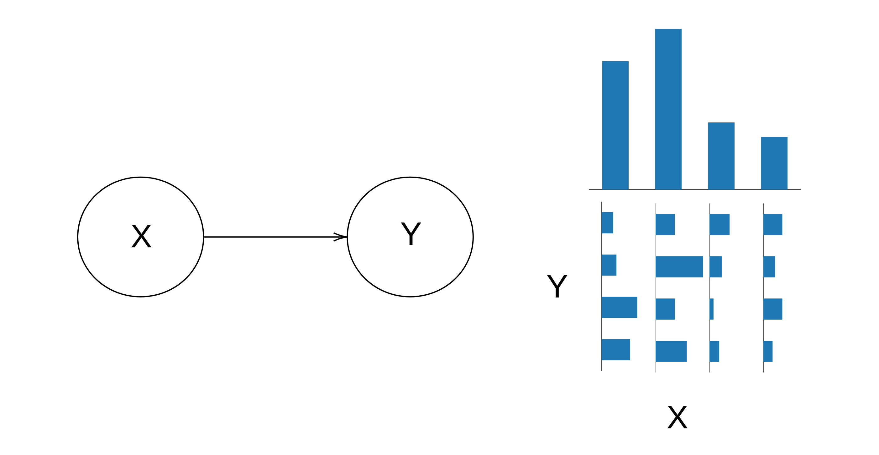
Then we abstract this by forgetting about Y: we just take $f(x,y)=x$.

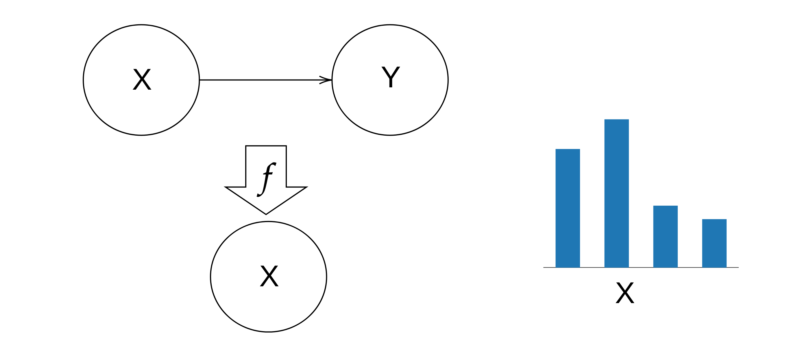
Now, if we want to go back to our original model, we can't recover the full distribution $P(X,Y)$, because we forgot about Y when abstracting. However, we know that the joint distribution must add up to our marginal distribution $P\left(X\right)$. So, what if we pick the set of all distributions that satisfy this property?

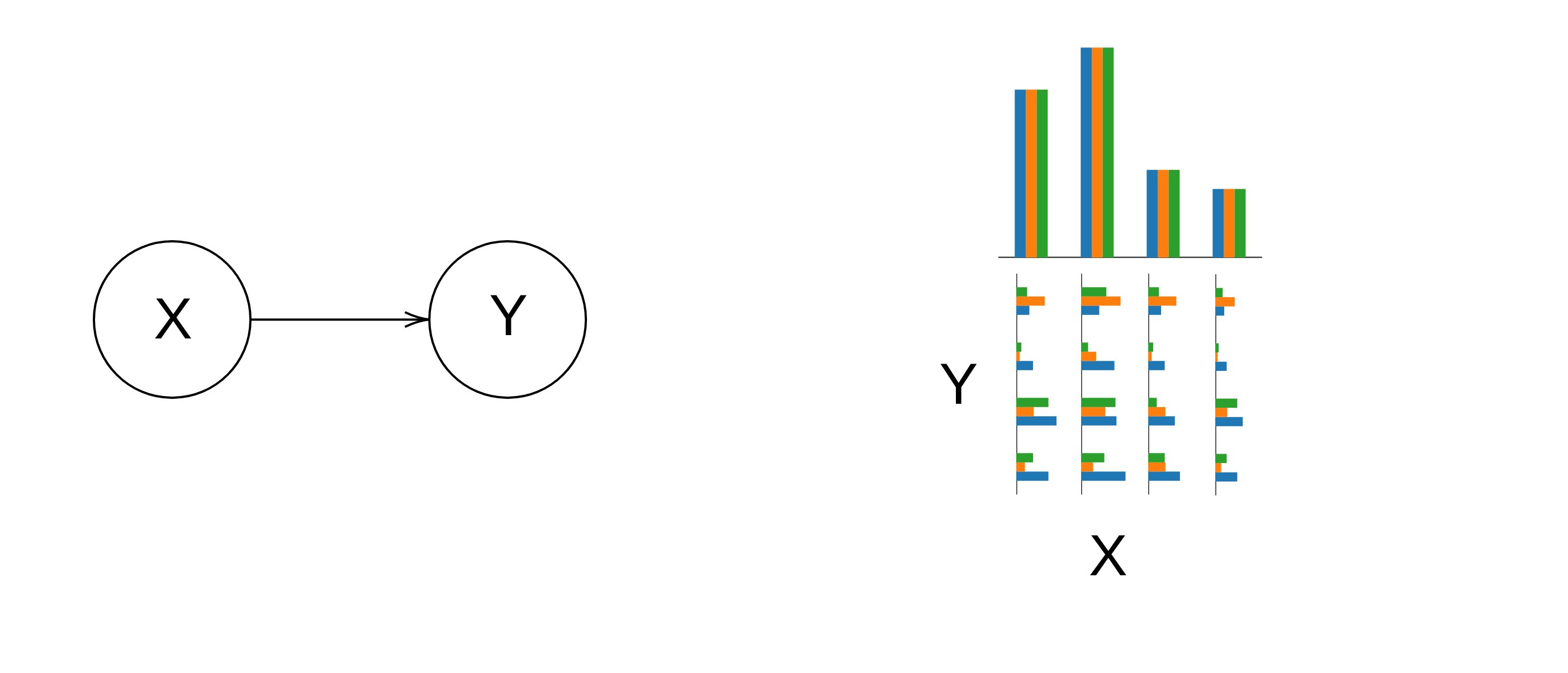
From this set of probability distributions we form our infradistribution. Let's call it $D$. Suppose we now pick a particular value $X=x$, and condition $D$ on $X=x$ (that is, we condition each of the distributions inside $D$ on $X=x$^[4]) and get a new infradistribution over $Y$, denoted $D(Y|X=x)$. Now, since we picked the set of all possible distributions compatible with $P\left(X\right)$, we know that $D(Y|X=x)$ must contain all possible probability distributions over $Y$: the set is maximal. There is nothing more we could add to it, and therefore it also contains zero information, since there is no scenario we rule out.^[5]

Infradistribution -> Abstraction:

Now, suppose we have a sharp infradistribution $D$ (that is, an infradistribution made only by probability distributions and not any weird measures) on a set $Z$. We can reverse-engineer the previous process to get an abstraction from it. Recall that in the previous section, the marginal probability $P\left(x\right)={\int }_{y\in Y}P(x,y)$ is the same for all distributions in the infradistribution and for all values $x$ of the abstracted model. 

Inspired by this, let's find the subsets of $Z$ that have the same probability on all of the distributions in $D$, that is, ${\int }_{z\in S}P\left(z\right)=p_S$ for all $P\in D$. Let's call these saturated subsets.

One obvious saturated subset is $Z$ itself, on which all the distributions have probability 1. Another is the empty subset. But that's not very useful. Suppose we find another saturated subset $S\subset Z$. Then the complement $\overline{S}$ must also be saturated, since it will have probability $1-p_S$ for all $P$ in $D$.

It follows that we can partition $Z$ into saturated subsets, which all have well-defined probabilities! Then it's clear how an abstraction arises, we just take the abstraction function $f$ to be $f\left(z\right)=S_z$, where $S_z$ is the saturated subset to which $z$ belongs. Let's see how this works with our previous example, where $Z$ is the set $X\times Y$:

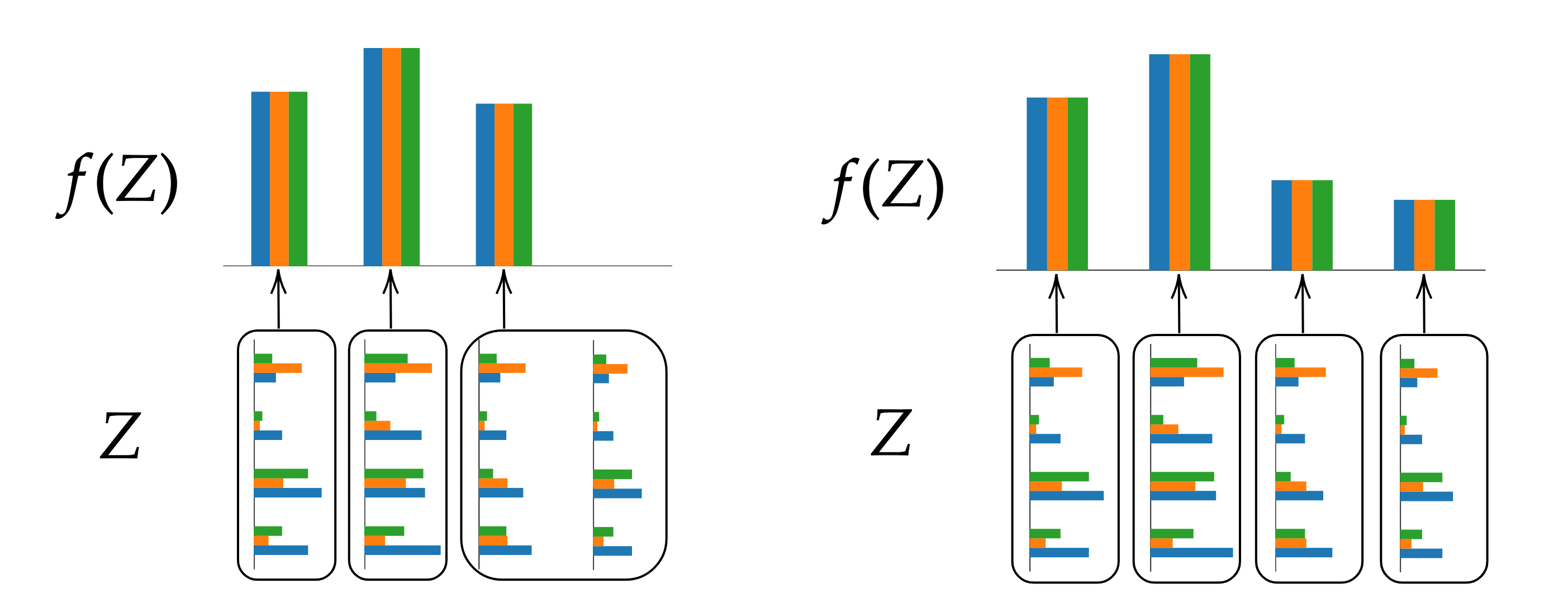
As we see, there is one problem: the same set admits multiple partitions. That's not really an issue, they just correspond to different abstractions, some more coarse-grained than others. For example, the abstraction on the left side of the image above corresponds to not only forgetting about Y, but also forgetting about the distinction between two of X's values.

There will always be a partition which is more fine-grained than all of the others. This corresponds to abstracting away the least information. If we go from an abstraction to an infradistribution and want to go back to the same abstraction, we'll have to choose the maximally fine-grained partition.

Now there is another issue. If you remember, in the previous section we noted that the infradistributions $D(Y|X=x)$ are maximal, in the sense that they contain all probability distributions over $Y$, and so contain zero informatoin. However, when building our abstraction, we haven't checked if D is maximal on the saturated subsets. If it is not maximal, then $D$ will have more information than $P\left(f\right(X\left)\right)$. So if we take the corresponding abstraction and then go back to an infradistribution, we will end up with a different infradistribution than we started with.

However, what do these non-maximal infradistributions mean? What happens if we have, say, only two or even one distribution on some saturated set?

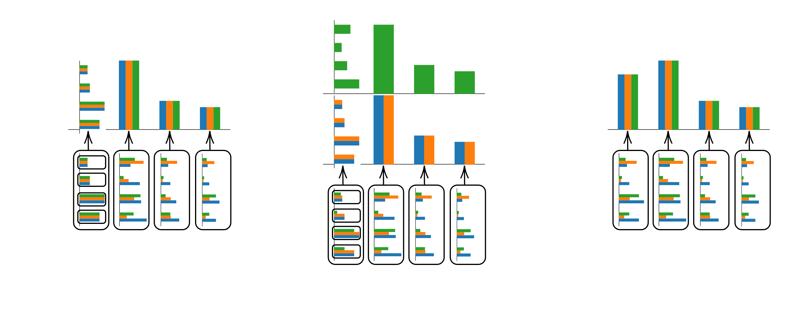
We have two extremal scenarios: in the maximal case, we have zero information and so abstract everything to a single probability distribution (right side in the image). In the minimal case, we just have one probability distribution, so all subsets of this set are saturated, and we are not abstracting anything (left side in the picture). In a middle case, the saturated set is neither maximal nor minimal. Then we can split $D\left(Y|x\right)$ into some number of infradistributions which have finer extremal partitions. The result is that instead of a single probability distribution on the abstracted set, we have an infradistribution.

Of course! The abstracted model might not have a fully specified probability distribution. It might itself have only an infradistribution. In the end infrabayesianism is a generalization of probability theory, so it has to be able to deal with the extra generality.

Final thoughts

All the examples above use finite discrete sets. However, both infrabayesianism and causal diagrams admit infinite sets and non-discrete topologies. Fortunately, infrabayesianism already has the tools to generalize the basic constructions I gave above.

The move from abstraction to infradistribution is just the pullback of the probability distribution in the abstract model along the abstraction function.

The reverse case is somewhat more complex. Once you have identified a partition, the abstracted probability distribution should just be the pushforward along the infrakernel^[6] given by $f\left(x\right)=\delta \left(\right[x\left]\right)$, where $\delta$ is the Dirac distribution. Unfortunately, this is not actually an infrakernel for nondiscrete sets since it's not bounded. I'm also not sure if partitions are the right way of thinking about this in the continuous setting.

1. ^{^}

   It might seem that adding more sets can't possibly help with our memory issues, but that depends on how the sets are represented. A bigger set can often be represented with a smaller data structure.

2. ^{^}

   The dual case are ultradistributions, in which you take the supremum to be maximally optimistic.

3. ^{^}

   This might be a bit confusing. See the "Motivating Sa-Measures" section of this post [? · GW] for an example.

4. ^{^}

   Normally conditioning infradistributions requires two steps, conditioning and then normalizing, but in this case all the distributions assign the same probability to the event X=x, so the normalization is just dividing everything by P(x) and doesn't really change anything.

5. ^{^}

   We could say informally that D(Y|X=x) is a "maximum-entropy" infradistribution. And I think if you sum all the constituent distributions in a reasonable way, you'd get the uniform distribution on Y. I wonder if this is a general principle, that is, the maximum entropy distribution always corresponds to the (normalized) infinite series of all probability distributions in the corresponding class.

6. ^{^}

   Infrakernels are basically functions along which you can push forward an infradistribution to get another infradistribution over a different set. See Definitions 13 and 17 here [? · GW].

0 comments

Comments sorted by top scores.