ParaScope: Do Language Models Plan the Upcoming Paragraph?

post by NickyP (Nicky) · 2025-02-21T16:50:20.745Z · LW · GW · 0 comments

Contents

  Short Version (5 minute version)
    Motivation.
    Brief Summary of Findings
  Long Version (30 minute version)
    The Core Methods
      Models Used
      Dataset Generation
  ParaScopes:
    1. Continuation ParaScope
    2. Auto-Encoder Map ParaScope
      Linear SONAR ParaScope
      MLP SONAR ParaScope
  Evaluation
    Baselines
      Neutral Baseline / Random Baseline
      Cheat-K Baseline
      Regeneration
      Auto-Decoded.
  Results of Evaluation of ParaScopes
    Scoring with Cosine Similarity using Text-Embed models
    Rubric Scoring
      Coherence Comparison
      Subject Maintenance
      Entity Preservation
      Detail Preservation
    Key Insights from Scoring
  Other Evaluations
    Which layers contribute the most?
    Is the"\n\n" token unique? Or do all the tokens contain future contextual information?
      Manipulating the residual stream by replacing "\n\n" tokens.
    Further Analysis of SONAR ParaScopes
      Which layers do SONAR Maps pay attention to?
    Quality of Scoring - Correlational Analysis
      How correlated is the same score for different methods?
      How correlated are different scores for the same method?
  Discussion and Limitations
    Acknowledgements 
  Appendix
    HyperParameters for SONAR Maps
      Linear Model
      MLP Model
    ParaScope Output Comparisons
    BLEU and ROGUE scores
None
No comments

This work is a continuation of work in a workshop paper: Extracting Paragraphs from LLM Token Activations, and based on continuous research into my main research agenda: Modelling Trajectories of Language Models [LW · GW]. See the GitHub repository for code additional details.

Short Version (5 minute version)

I've been trying to understand how Language models "plan", in particular what they're going to write. I propose the idea of Residual Stream Decoders, and in particular, "ParaScopes" to understand if a language model might be scoping out the upcoming paragraph within their residual stream.

I find some evidence that a couple of relatively basic methods can sometimes find what the upcoming outputs might look like. The evidence for "explicit planning" seems weak in Llama 3B, but there is some relatively strong evidence of "implicit steering" in the form of "knowing what the immediate future might look like". Additionally current attempts have room for improvement.

Motivation.

When a Language Model (LM) is writing things, it would be good to know if the Language Model is planning for any kind of specific output. While the domain of text with current LMs is unlikely to be that risky, they will likely be used to do tasks of increasing complexity, and may do things that may increasingly be described as "goal-directedness [AF · GW]" by some senses of the word. 

As a weaker claim, I simply say that LMs are likely steering, either implicitly or explicitly, towards some kinds of outputs. For some more discussion on this, read my posts on Ideation and Trajectory Modelling in Language Models [AF · GW].

We say that the language model is steering explicitly towards certain outcomes, if the model is internally representing some ideas of what longer-term states should look like. If given the same input prompt and context, the model should reliably try to steer towards some kinds out outputs, even if perturbed.

We say the language model is steering implicitly, if the language model does NOT have an explicit representation of what the end states might look like, but is rather following well-learned formulas to go from the current state to the next. This means that the model has some distribution of output states that are likely, but if perturbed, may go down some other path instead.

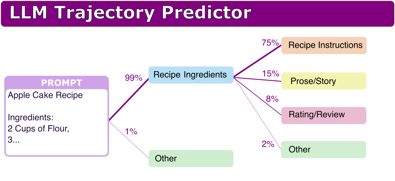
My original plan before I reached these results, was that it would be quite good to be able to map some distribution of what possible future outcomes might look like. Here is a visualization:

The experiments here so far only work on understanding what internal "immediate next step" planning might be going on in the model, and are probably more in-line with implicit steering rather than explicit steering. The results as follow show the current methods I have tried, with promising initial results despite not that much work being done. I expect with further work these ideas could be refined to work better.

 

Brief Summary of Findings

We suggest two kinds of Residual Stream Decoders that try to reveal to what degree the Language model is planning the upcoming paragraph (where ParaScope = "Paragraph Scope"): 

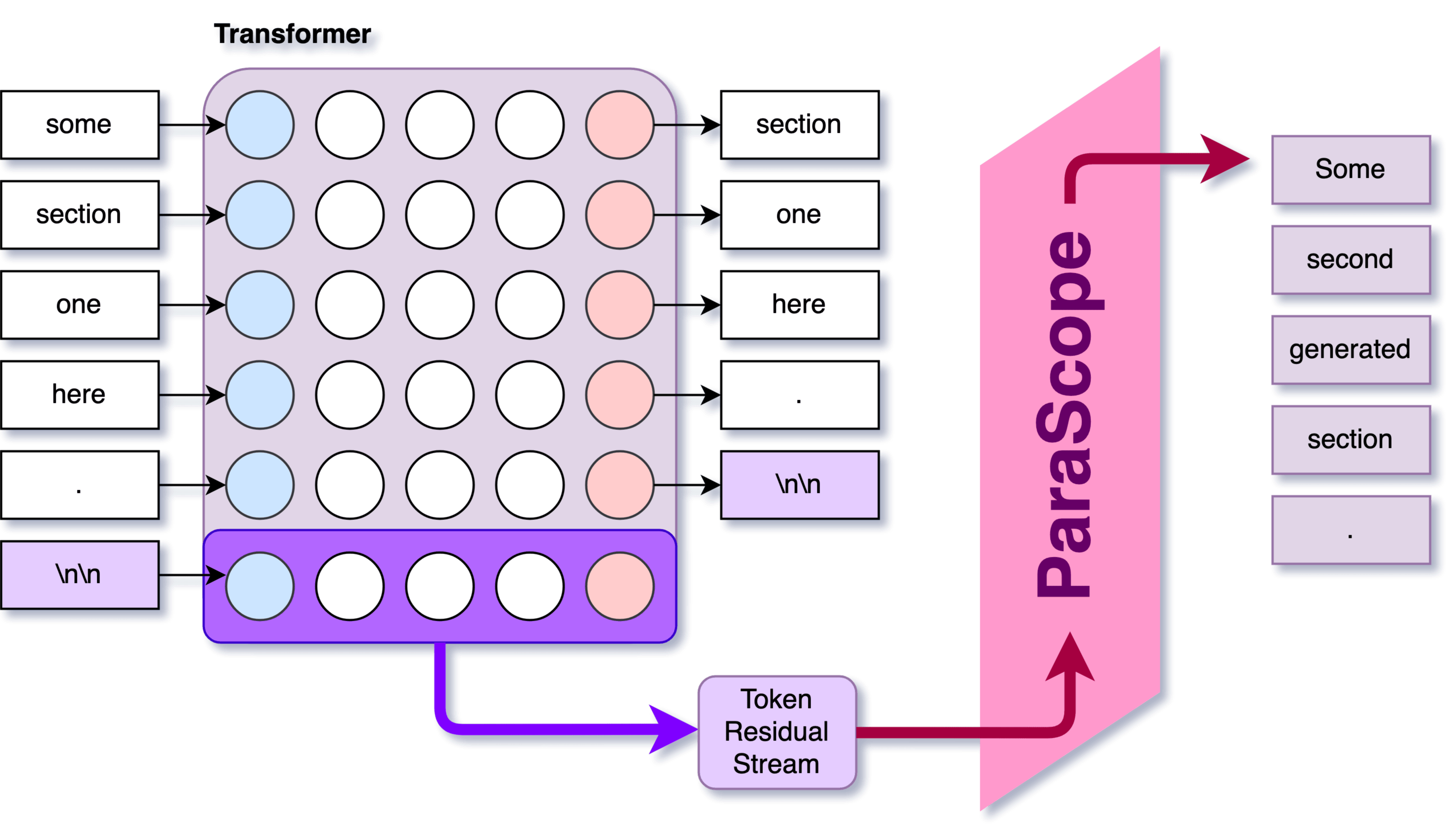
1. The Continuation ParaScope is a straightforward approach that takes the residual stream from a "\n\n" token and uses it as context for continued generation, testing whether the model can recover the intended next paragraph.
2. The AutoEncoder Map ParaScope takes a more sophisticated approach by mapping the residual stream to Text AutoEncoder Embeddings using a trained map (Linear or MLP), then decoding it back to text.

Both methods demonstrated performance comparable to having five tokens of "cheat" context, suggesting that language models seem to "plan" or "keep context of" at least that far in advance.

SONAR ParaScope and Continuation ParaScope showed different strengths in their performance. SONAR ParaScope performed better at maintaining broad subject matter (83.2% vs 52.5% similar field or better), while the Continuation ParaScope was typically more coherence, being more often at least partially coherence (96.7% vs 72.2%).

These results significantly outperformed the random baseline (which achieved only 5.0% bread subject alignment), while falling well short of the full-context regeneration baseline (which achieved 99.0% broad subject alignment).

Additionally, a (very brief) analysis of the model's layers seems to indicate that the middle layers (60-80% depth) had the strongest impact on generation. 

Lastly, we found some evidence that that models we looked at typically avoids thinking about the next paragraph until the last moment, with the "\n\n" token typically marking the beginning of next-paragraph information encoding. 

We hope that this work can be expanded on the build better understanding of the degree of internal-planning in Language Models, and help us assess and monitor Language Model behaviour.

 

Long Version (30 minute version)

The Core Methods

We know transformers process text token-by-token, but I intuitively feel they must be doing some form of planning to maintain coherence. I wanted to test a specific hypothesis: that significant information about an upcoming paragraph is encoded in the residual stream of the newline token that precedes it. 

To investigate this:

1. I generated a dataset of Language-Model-Generated text with relatively clear transitions. (This mostly just excludes "code").
2. I tried a couple of ways of extracting information from the residual stream at the transition token

I coin the following terms:

• Residual Stream Decoder:  Approaches that try to broadly decode information from the residual stream into human-readable form.
• ParaScopes: (Paragraph Scope): Methods that attempt to decode paragraph-level information from the the residual at a single token. The focus will be on the transition between paragraphs, but I also run some experiments arbitrary tokens within a text.

Here I propose two simple ParaScope methods, detailed in more depth below:

1) Continuation ParaScope: Continuing generation with the original model where the residual of the token to be decoded as context.

2) Text Auto-Encoder Map ParaScope: Training a map from residual stream to the embedding space vector generated by a Text Auto-Encoder [LW · GW] model (the input to the Text AutoEncoder's Encoder is the desired paragraph), then using the decoding the embedding vector with the AutoEncoder's Decoder.

For the text, we use the SONAR text auto-encoder, as it seems to be the best from my brief analysis [LW · GW],  

 

Models Used

The model I used for experiments was Llama-3.2-3B-Instruct. The small model makes it inexpensive to run for large numbers of samples. All generation with Llama use temperature=0.3.

Additionally, I used SONAR embedding models as the language model auto-encoder.

I used all-mpnet-base-v2 as the text-embed comparison model.

 

Dataset Generation

The key challenge was getting clean paragraph transitions that would let us study how models encode upcoming content. In previous attempts at "dataset creation", I often had issues with lack of diversity. My latest solution is a two-stage process:

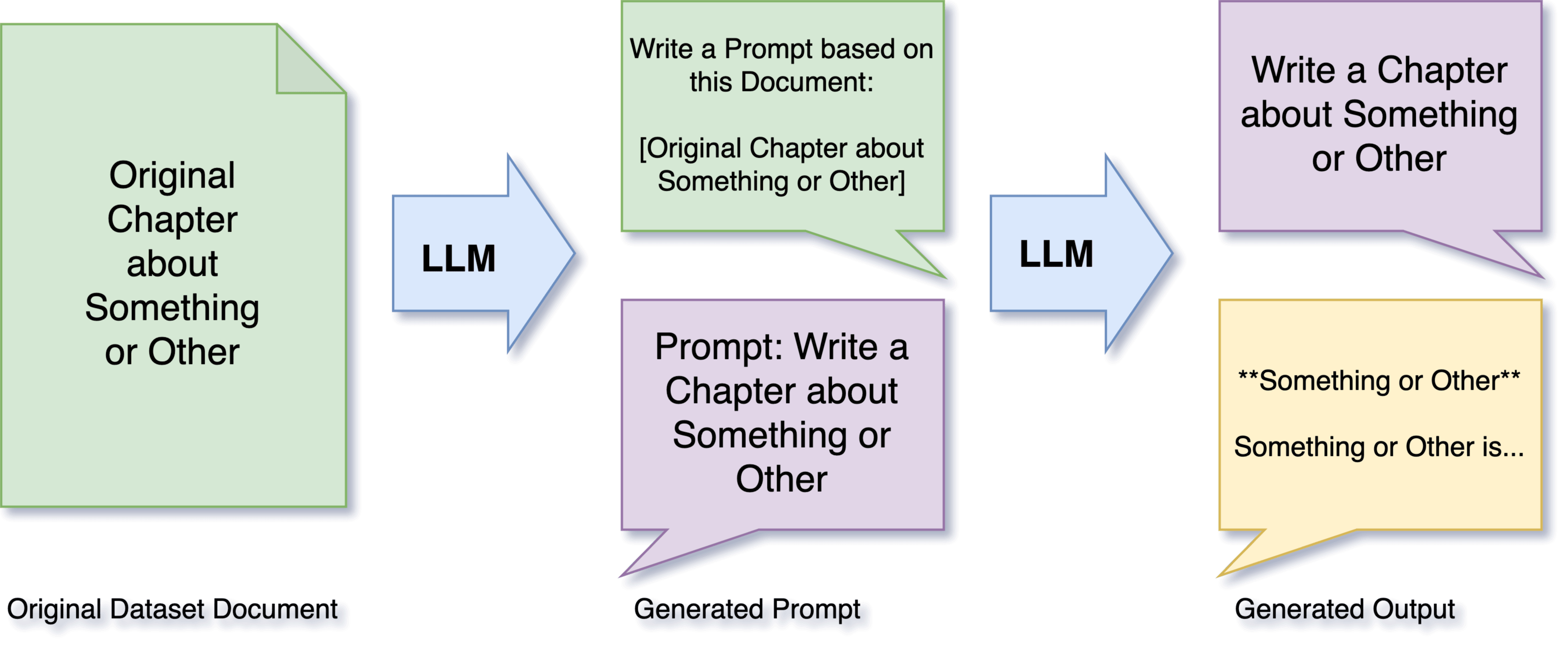
First stage (prompt generation):

• Take chunks of text from RedPajama's CommonCrawl
• Ask Llama 3.2-3B to convert each chunk into a writing prompt
• Format: "Write a [type], titled [name], which includes [topics], approximately [length]"

Second stage (content generation):

• Feed these prompts back to the same model architecture
• Collect the generated paragraph pairs
• Filter for transitions (with "\n\n" tokens)

Why this approach: By getting text generated by the LLM we want to study, we have a guarantee that the model was actually pretty likely to generate the upcoming paragraph. If we used an existing dataset, then we would have much weaker guarantees.

In total, I generated 100,000 responses, which splits into approximately 1M "paragraphs" when split into by occurrences of "\n\n". I used a split of 99% train, 1% test.

For more details, see the GitHub Repository, or view the dataset on HuggingFace Hub.

 

ParaScopes:

We want to test the degree to which the residual stream has information about the whole upcoming paragraph, not just the next token. To do the residual stream decoding, we first collect the residual stream activations at the transition points. That is, we:

• Take a original language model on some text.
• Insert the a whole prompt + generated text into the language model.
• Save the residual stream at all the occurrences of "\n\n" into "paragraphs".
  • I took the "residual diffs", including both the MLP and Attention layer outputs. This has a large dimensionality (2 x 28 layers x 3072 dimensions = 172,032 total dimensions)

Our task now is to be able to translate each transition token's residual stream activations into the next paragraph of text. 

 

1. Continuation ParaScope

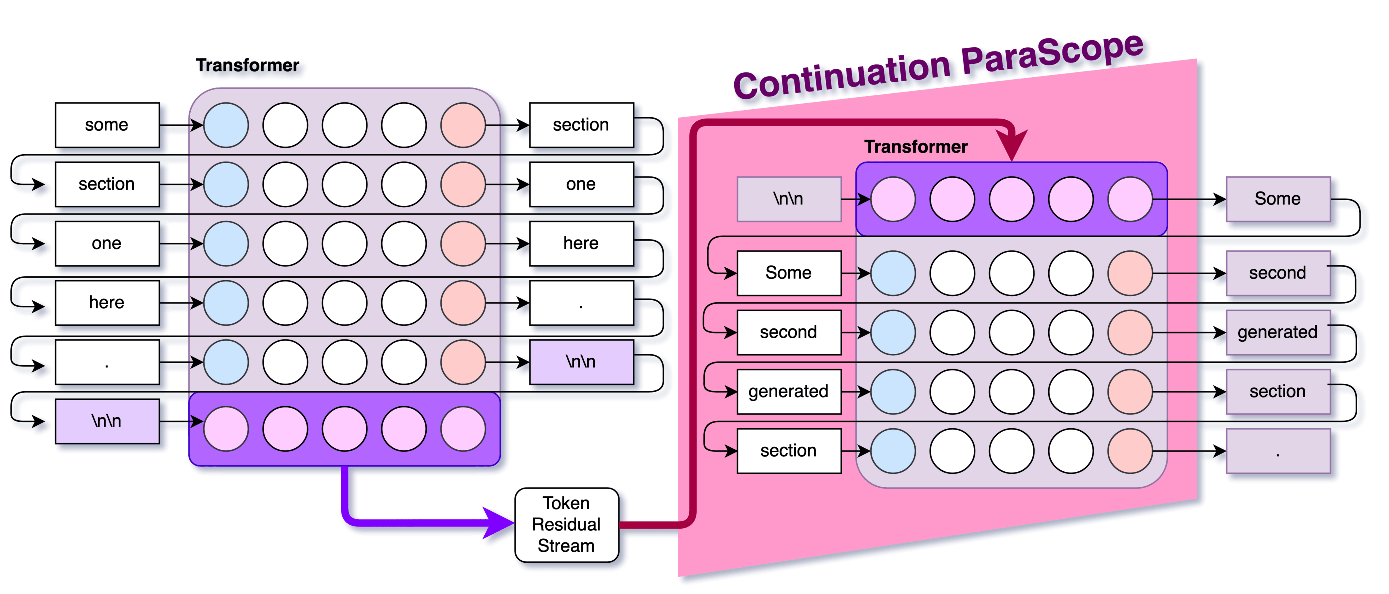
The continuation ParaScope is probably the least complicated, has no hyper-parameters, and was what I used in my Extracting Paragraphs paper. The core idea:

• Insert a blank prompt of <bos>\n\n to the model
• Intervene on the activations of \n\n to be the saved activations of the residual stream
• Generate what comes next.

We then compare to the baselines and the "Continuation ParaScope" paragraphs to see how well we managed to decode the residual stream.

 

2. Auto-Encoder Map ParaScope

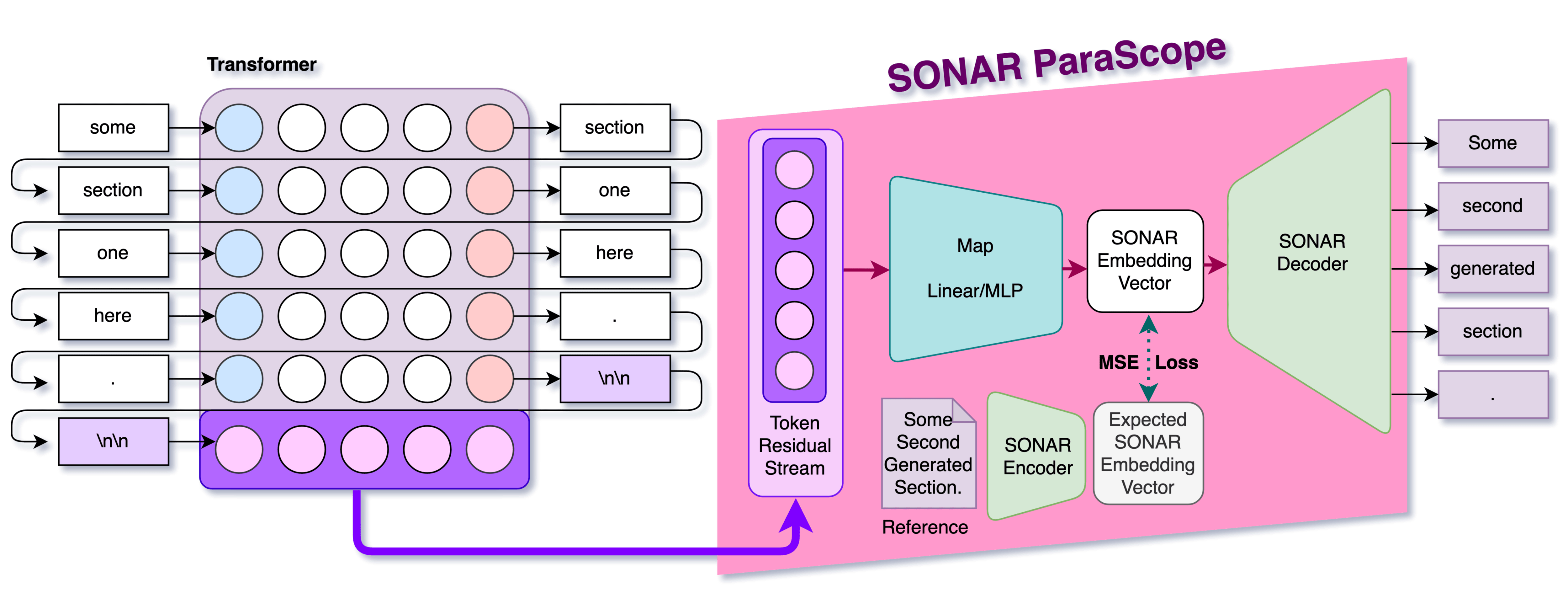
The AutoEncoder Map ParaScope consists of two stages:

• A map that takes in the residual stream and outputs the approximate auto-encoder embeddings vector
• The decoder that takes the embeddings vector and returns some text. 

In this post, we use SONAR as the text auto-encoder. SONAR is a text-embed auto-encoder that was trained for purposes of machine translation. The key property it has over almost all other text-embed models, is that it comes not only with an encoder, but also a decoder.

Thus, one can pass in a short passage, encode into a vector of size 1024, then later decode that vector to get a passage that should be an almost-exact match to the original passage. Read this post on Text AutoEncoders [LW · GW] if you want more details.

 

 

As we will mostly stick to using SONAR, we will mostly refer to the AutoEncoder Map ParaScopes as SONAR ParaScopes.

For training the residual-to-sonar map, we:

• Take the residual stream activation of the "\n\n", and normalize them.
  • I "assumed" each dimension as being independent, and offset by mean + and dividing by stdev for that dimension throughout all the data. This step could possibly be improved.
  • This is the input to our map
• Take the next paragraph
  • We take the entire paragraph, embed it using SONAR Embed model to get an embedding vector of size 1024.
  • The embedding vectors are also normalized by mean + stdev.
  • This is the expected output of our (MLP or Linear) map
• We train the simple translation map from residual-stream-inputs to sonar-embed-outputs using Mean Squared Error loss.

We train two types of maps: 

Linear SONAR ParaScope

1) The Linear map takes the normalized residuals of the first 50% of residual diffs, and outputs a normalized sonar vector, but basically: Normalize( n_layers * d_model ) → d_sonar = 1024

MLP SONAR ParaScope

2) The MLP map additionally has two hidden layers of size 8192. See Appendix^[1] for hyper-parameters, but basically: Normalize( n_layers * d_model ) → GeLU( 8,192 ) → GeLU( 8,192 ) → 1,024

 

Evaluation

Baselines

In order to see how good our ParaScope probing methods are, we need some baselines to compare against. We choose a various few baselines:

Neutral Baseline / Random Baseline

For this, we simply generate with the model being given a blank <bos>\n\n context, no interventions. This should work pretty poorly, but will give a lower bound for how bad our methods could be

Cheat-K Baseline

For this, we let the model do the baseline generation, but let the model generate with a few tokens of the upcoming section revealed for context. For example, if the original section was ** Simple Recipe for an Organic One-Pot Pumpkin Soup **, for cheat-1, we would input: <bos>\n\n**, for cheat-5 we would input <bos>\n\n** Simple Recipe for an. 

For sake of "fairness" of comparisons, filtered examples where more than 50% of the text was exposed (that means, for cheat-10, it must be at least 20 tokens long).

We use cheat-1, cheat-5, and cheat-10 as our comparisons.

Regeneration

Another thing we can compare against is taking the whole previous context: prompt + previously generated sections, and using the model to generate what could have come next again (again, with temperature=0.3). This gives us the real distribution, and is what we want to match

Auto-Decoded.

Finally, another method for comparison is to take the reference text, encode it using SONAR, and then decode it again using SONAR. As SONAR is not perfectly deterministic, it should give some idea of what the limitations might be.

 

Results of Evaluation of ParaScopes

There were a few main ways of evaluating the ParaScopes of the residual stream:

• Manually look at some text examples (see: Appendix^[2], GitHub)
• Compare using text-embed models
• Traditional metrics like BLEURT (or older BLEU and ROGUE)
• Compare using LLM with rubric scoring

Each has their pros and cons. None of them really give a complete picture, but I think the LLM rubric scoring seems to work the best of them. 

 

Scoring with Cosine Similarity using Text-Embed models

The simplest way to compare the texts, is to use a text-embed model, and compare the embedding vector using cosine-similarity against the reference text (we used all-mpnet-base-v2, a relatively small text embed model). 

Here, the Linear and MLP ParaScope models seem to work almost identically well, with perhaps a tiny edge to the MLP model. Both seem better than the ParaScope continuation by about ~0.2 in cosine similarity on average. They seem comparable to the "cheat-5" baseline.

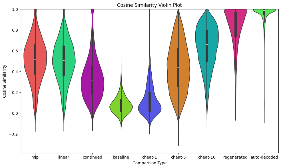
	mlp	linear	cont.	base.	c-1	c-5	c-10	regen.	auto.
Mean	0.51	0.50	0.33	0.08	0.12	0.44	0.63	0.82	0.95
StDev	±0.20	±0.20	±0.20	±0.08	±0.14	±0.23	±0.20	±0.19	±0.13

This is fine and all, but I don't find the scores particularly easy to understand. It seems like maybe ParaScope Linear/MLP are better but hard to tell. Here is a table of ths scores:

 

Additionally, I try with BLEURT score, which is also an imperfect metric, but better than the BLEU or ROGUE scores (see Appendix for those^[3]) but still shows results mostly consistent with "around the same level as cheat-5, worse than regeneration". We see regeneration suffers here more compared to Auto-decoded. I still think these results are not that meaningful. 

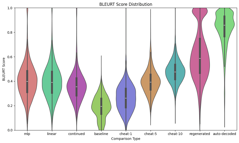
Metric	mlp	linear	cont.	base	c-1	c-5	c-10	regen.	auto
Mean	0.404	0.395	0.364	0.192	0.263	0.396	0.477	0.619	0.825
StdDev	±0.144	±0.138	±0.135	±0.094	±0.107	±0.102	±0.093	±0.216	±0.145

 

Rubric Scoring

To do a more fine-grained evaluation, I also scored the outputs using GPT-4o-mini with a rubric for different aspects of the text. This procedure was somewhat tuned until it was mostly consistent at giving scores that match my intuitions.

In particular, one thing that helped get reliable scoring, was to ask the model to first give brief reasoning about the scoring, of format that is "[reasoning about text], Thus: [explicit name of score which applies]: Thus: out of [max score], score X"

A TLDR of the axes which showed the most interesting results:

• Coherence (0-3)
  • 0: Incoherent (nonsense/repetition) | 1: Partially coherent (formatting issues) | 2: Mostly coherent (minor errors) | 3: Perfect flow (logical progression)
• Subject Match (-1 to 4)
  • -1: No subjects | 0: Unrelated ("law" vs "physics") | 1: Similar field (biology/physics) | 2: Related domain (history/archaeology) | 3: Same subject (ancient mayans) | 4: Identical focus (mayan architecture)
• Entities (-1 to 4)
  • -1: No entities | 0: Unrelated (Norway/smartphone) | 1: Similar category (countries/people) | 2: Related entities (similar countries) | 3: Partial match (some identical) | 4: Complete match (all key entities identical)
• Details (-1 to 3)
  • -1: No details | 0: Different details | 1: Basic overlap ("anti-inflammatory") | 2: Moderate match (benefits + facts) | 3: Specific match (exact percentages)

For a full breakdown of the rubric, as well as additional metrics collected, see the github.

What we mostly see is that the MLP and Linear SONAR ParaScope methods seem to work almost identically well, and there are different tradeoffs between Sonar ParaScopes and Continuation ParaScope.   

 

Coherence Comparison

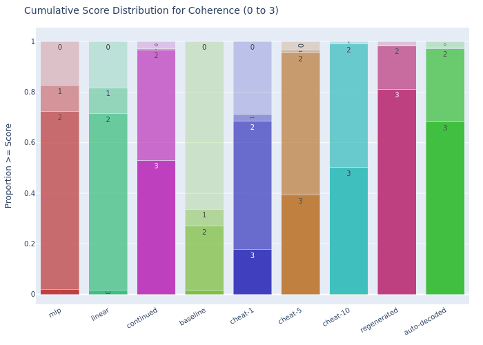
SONAR ParaScope: Achieves 72.2% partial coherence (Score 1+) but only 1.9% mostly coherent (Score 2), performing just slightly above cheat-1 baseline (68.4% Score 1+) and far below other baselines.

Continuation ParaScope: Reaches 96.7% partial coherence (Score 1+) and 53.0% mostly coherent (Score 2), performing similarly to cheat-10 (98.9% Score 1+, 50.2% Score 2).

The regenerated baseline achieves 98.3% partial coherence and 81.2% mostly coherent, showing room for improvement particularly at higher coherence levels.

 

Subject Maintenance

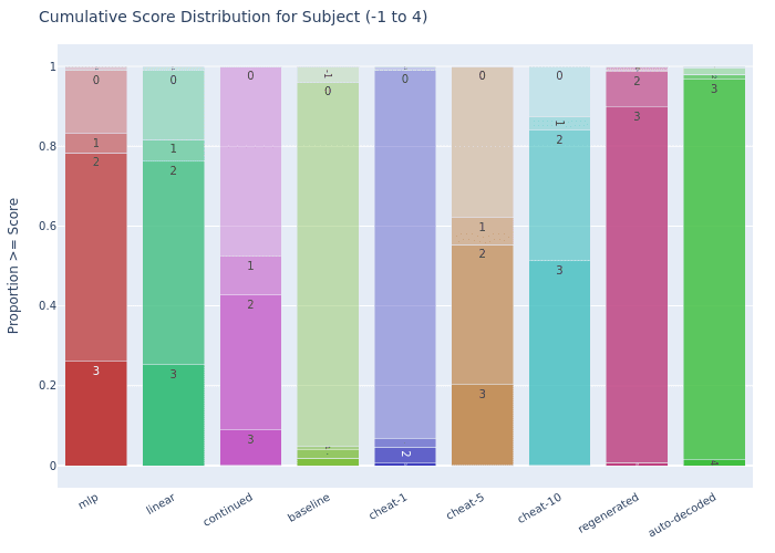
SONAR ParaScope: Shows strong topic relevance with 83.2% similar field or better (Score 1+) and 78.3% related domain or better (Score 2+), outperforming even cheat-10 (84.0% Score 1+, 51.3% Score 2+).

Continuation ParaScope: Achieves 52.5% similar field or better (Score 1+) and 42.7% related domain or better (Score 2+), performing slightly below cheat-5 (62.2% Score 1+, 55.3% Score 2+).

The regenerated baseline almost always achieves similar field 99.0% (score 1+) and related domain 98.65% (Score 2+), indicating there is significant room for improvement, but that they significantly outperform the random baseline which only gets 5.0% score 1+.

 

Entity Preservation

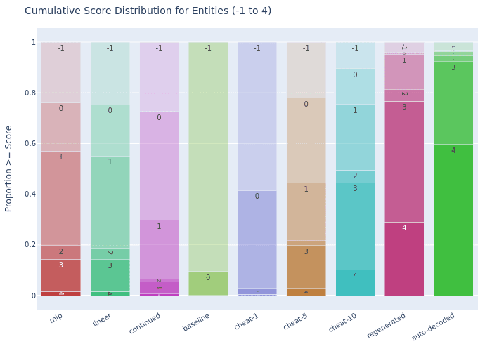
SONAR ParaScope: Maintains 57.1% similar category or better (Score 1+) and 19.7% related entities or better (Score 2+), performing between cheat-5 (44.4% Score 1+) and cheat-10 (75.5% Score 1+).

Continuation ParaScope: Shows 29.7% similar category or better (Score 1+) and 6.4% related entities or better (Score 2+), falling well below cheat-5 performance (44.4% Score 1+).

 

Detail Preservation

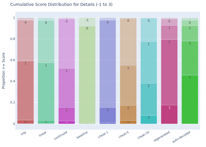
SONAR ParaScope: Reaches 59.2% basic overlap or better (Score 1+), similar to cheat-5 (54.9%), but drops to 3.6% moderate match or better (Score 2+), well below cheat-5 (17.2%).

Continuation ParaScope: Achieves 52.3% basic overlap or better (Score 1+) and 15.4% moderate match or better (Score 2+), performing close to cheat-5 levels (54.9% and 17.2%

 

 

Key Insights from Scoring

The methods show clear complementary strengths: SONAR better preserves broad semantic relationships despite training mismatch, while continuation maintains better coherence and specific details. Performance against baselines reveals significant room for improvement, particularly in entity and detail preservation.

Overall, the ParaScopes seem to be similar in quality to cheat-5 generations.

SONAR ParaScope coherence issues likely stem from its training objective (MSE) and could be improved through better loss functions (using CE Loss of decoded outputs) or fine-tuning SONAR to better handle the noise we have here. There are likely also other improvements one could do for the residual-to-sonar maps.

Continuation ParaScope issues seem to mostly stem from not being able to cling onto the information that it has it's context. It's possible that re-scaling the activations from the transferred activations to be more dominant, or allowing multiple generations and doing some kind of "Best of" generation would show better results.

---

Other Evaluations

Some questions remain. In particular, one question to try understand, is how far ahead this "context building" or "planning" might be occurring? I try to find out by testing Continuation ParaScope on different close to the transition token "\n\n", and also try to see how what layers of the model might this "planning" be occurring in.

To do these more specific evaluations, I used a narrower dataset, as was used in the original "Extracting Paragraphs" paper. That is, we had 20 types of outputs, which were specifically of the form "Write a paragraph about X, then write a a paragraph about Y. Do not mention X or Y explicitly.". This makes it easier to control that the next paragraph is different to the previous, and also prevent the model from over-fitting on the first token of the output typically naming X or Y. 

Additionally, I ran the tests on Gemma-2-9B-it instead of Llama-3.2-3B-Instruct. This is because the smaller 3B model usually struggled to do the task of talking about X without naming X.

 

Which layers contribute the most?

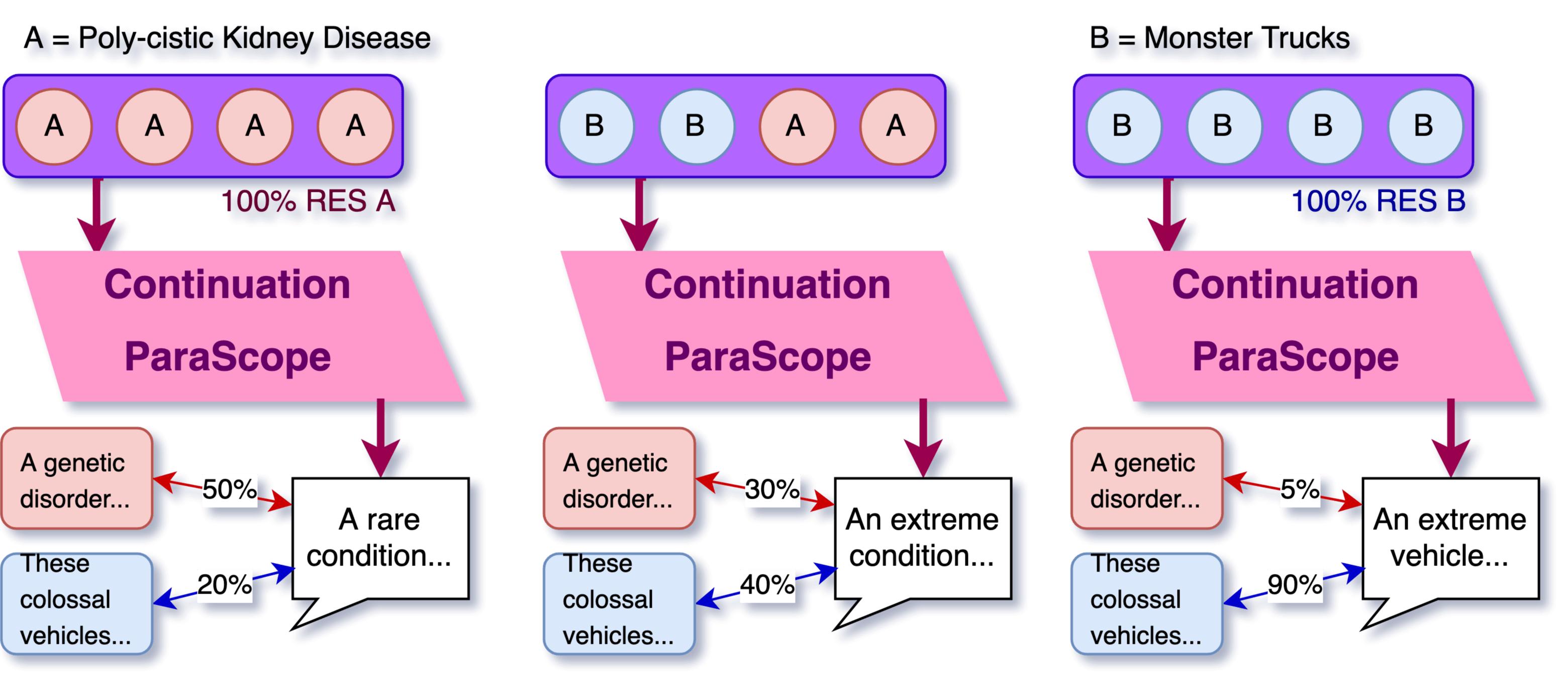
I try doing a basic form of "Layer Scrubbing" to find what layers are used. For this part, I only used a single comparison example A vs B, where:

• Prompt = Tell me about cleaning your house in 50 words, then tell me about [A or B] in 50 words. Structure it as 2 paragraphs, 1 paragraph each. Do NOT explicitly name either topic.
• initial paragraph = "write about cleaning your house"
• possible paragraph A = "poly-cystic kidney disease"
• possible paragraph B = "monster trucks"

The "Layer Scrubbing" then involved replacing the Whole residual stream activations at different layers (not just the differences):

• Get the activations of residual stream of "\n\n" token for RES A: [Prompt A + Initial Paragraph] and for RES B [Prompt B + Initial Paragraph]
• For each K between 0 and N:
  • Generate a Continuation ParaScope, which takes the first 1...K layers from RES A and the final K+1...N layers from RES B.
  • Repeat this 100 times and save all of them
  • Generate the Reverse also: take the first 1...K layers from RES B, and final K+1...N Layers from RES A
  • Repeat this 100 times and save all of them
• The evaluation then involved:
  • Take the generated outputs for ALL values of K, and compare the output against a full-context generated reference output A and reference output B using a semantic text-embed model: all-mpnet-base-v2.

I found that generating a single output was quite noisy, and so to ensure that we are measuring "information available" rather than "probing quality", I ran each continuation 64 times, and got the best result when comparing against A and against B.

Below, we see the results, comparing the cosine similarity of the outputs with different layer scrubbing:

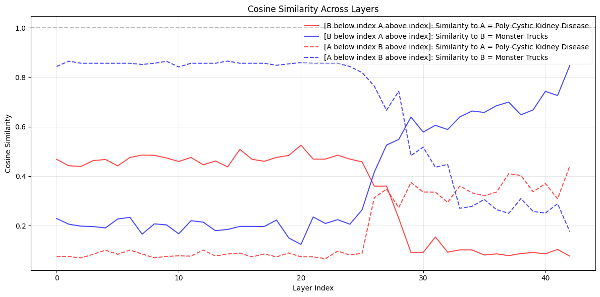
From this, we can see that the first 25 layers out of 42 have little effect on generation, whereas between layer 25 and 35 makes a huge to the output, and we also see a significant jump at the final layer, as when this is replaced, the "output embeds" get replaced and the first generated token changes.

I will need to more thoroughly test this by using more than a single pair of examples, but overall, this seems somewhat in line with other research showing middle layers having more of the impact on "high level" thinking. 

 

Is the"\n\n" token unique? Or do all the tokens contain future contextual information?

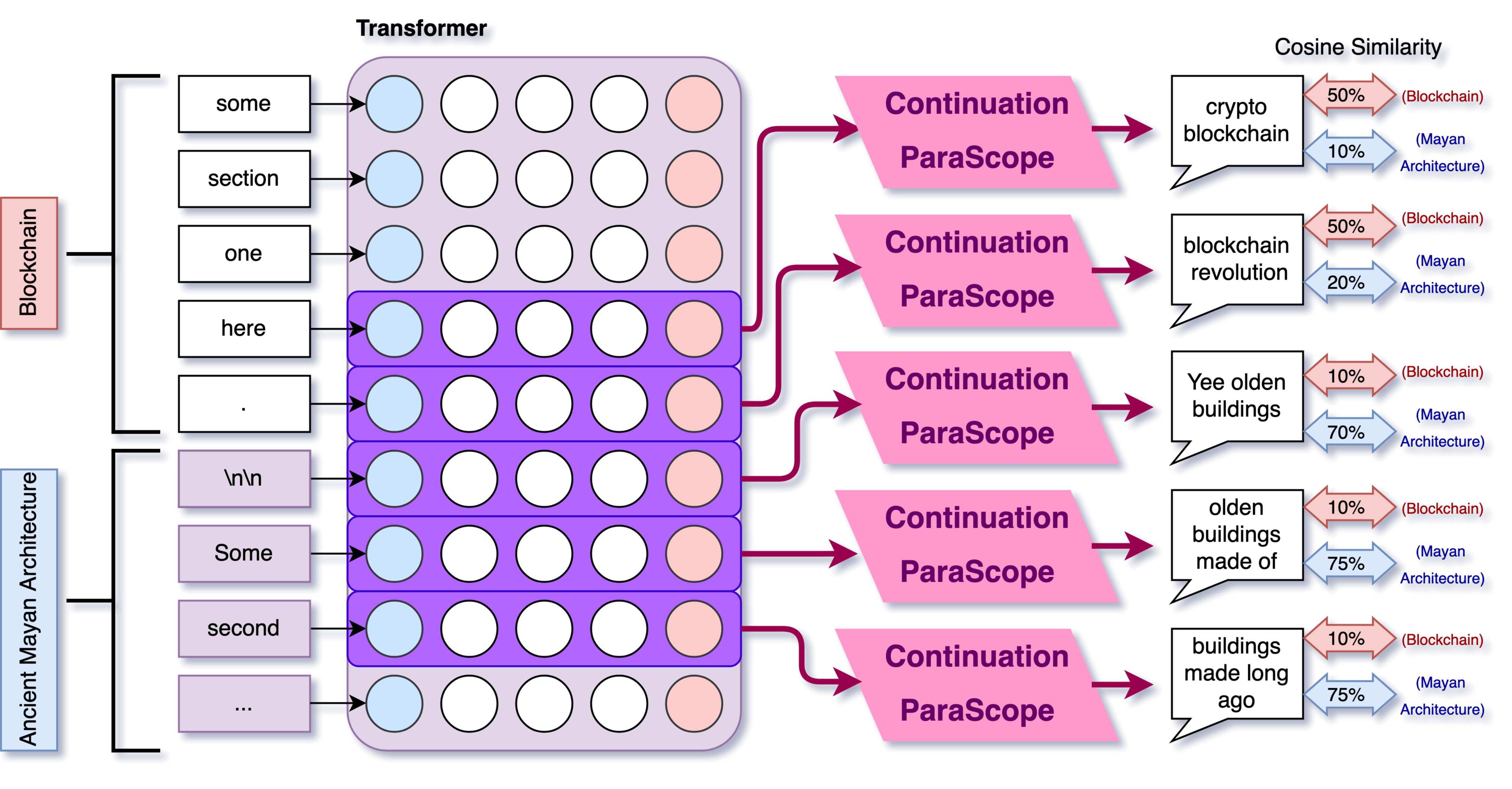
How much do different tokens include information about the upcoming paragraph? How does it differ before vs after the paragraph begins generation? We try using the "Continuation ParaScope" on the residual stream of tokens within a range of the transition "\n\n" token. More specifically, the procedure is:

• We give Gemma-2-9B a prompt like: "Write about blockchain, then write about Ancient Mayan Architecture". The output will be something like:
  • Topic 1: This revolutionary technology functions as a decentralized and immutable digital ledger.  Information is recorded in \"blocks\" that are linked together chronologically, creating a transparent and secure chain of transactions.  \n\n
  • Topic 2: Ancient civilizations left behind impressive structures, often built with intricate stonework and astronomical alignments.  These monumental creations served as religious centers, palaces, and observatories, showcasing the advanced knowledge and engineering skills of their builders.
• Get the residual stream of tokens close to "\n\n", including some from both topics:
  • creating a transparent and secure chain of transactions.  \n\n Ancient civilizations left behind impressive structures, often built
• Use Continuation ParaScope to see what the model might generate 64 possible completions at each of these tokens. Here is what these might look like:
  • " transparent" -> "and secure system for..."
  • "." -> "\n\n This revolutionary technology is..."
  • "\n\n" -> "Ancient structures built"
  • "impressive" -> "structures built long ago"
• Compare these outputs against the original using text-embed model. We use all-mpnet-base-v2 again for this. This is imperfect since we compare the start of paragraph 1 with a potential continuation of paragraph 1, while we compare paragraph 2 with a potential start of paragraph 2.

 

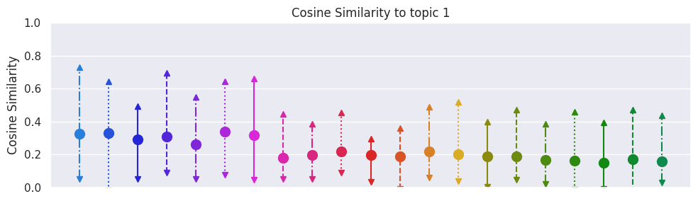
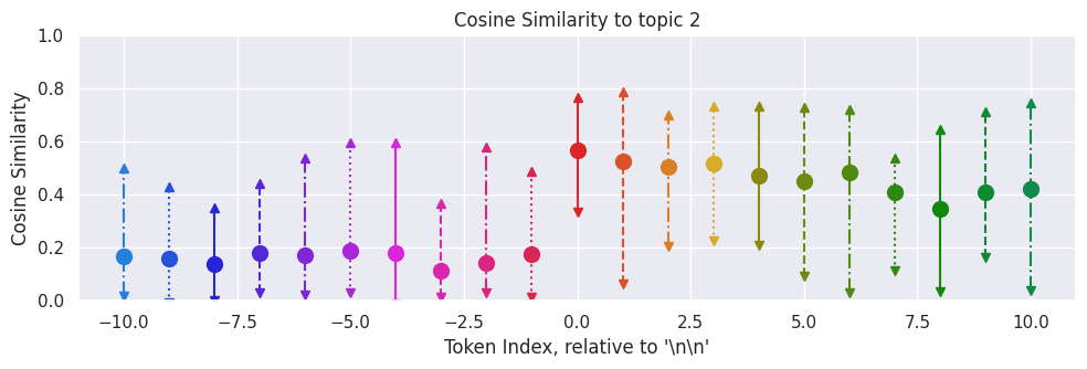
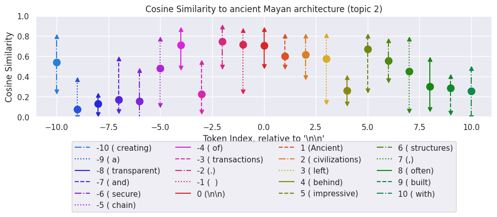
Here is an example between two specific texts (blockchain vs ancient mayan architecture):

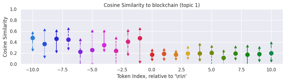
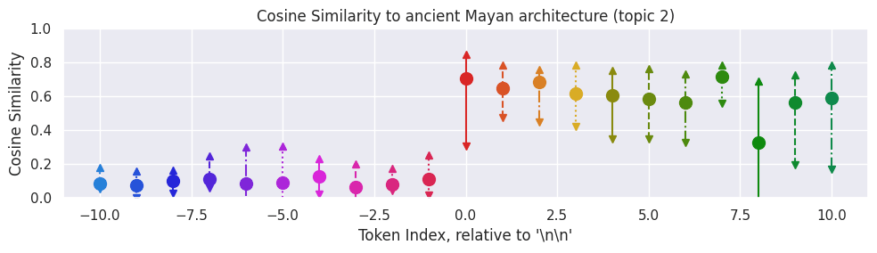
We can see that before the "\n\n" token, the model basically never outputs anything even vaguely similar to "ancient Mayan architecture", and often outputs things that are somewhat similar to the blockchain paragraph. After the newline, it consistently outputs things that are judged to be very similar to ancient Mayan architecture and dissimilar to blockchain.

 

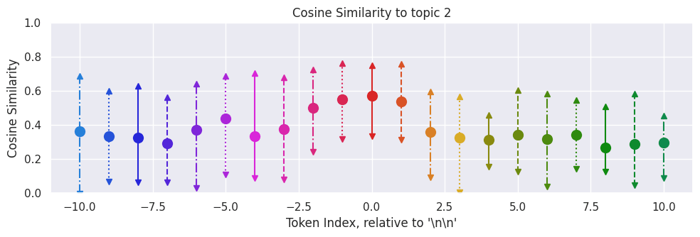
How does this fare if we average across the 20 text example that we have? We see results below:

This seems to indicate that the "\n\n" token seems to be when the model starts thinking about the next paragraph, but not when it stops. The similarity to topic 1 is not that high, even before the "\n\n", likely indicating that the metric against topic 1 seems to be poor, but the results for for topic 2 show a clear transition.

From these basic experiments, it seem that it is not exclusively the "\n\n" token that has enough contextual information to get a good grasp of the output. It more seems like the "\n\n" token is simply the first of many tokens to contain information about the upcoming paragraph. Tokens before seem to contain very little, whereas tokens after seem to contain the same or more information about paragraph.

This poses that it may be challenging if one might be interested in observing what future outputs might be like before we reach them

 

Manipulating the residual stream by replacing "\n\n" tokens.

We can also try see how the model deals with scenarios where we insert a "\n\n" token randomly before the end of the generation. That is, consider we have a text with two paragraphs, that start and end like such:

• I like toast because it is very yummy.\n\n
• Extreme machines that people like to watch crushing things.

We can instead insert a "\n\n" at some point mid sentence. For example:

• I like toast because\n\n.

One might expect two main things to happen. Either the model notices the early "\n\n" and tries to recover, to get back the original text but continued. Alternatively, the model might think that the paragraph is done, and that the model can continue.

If we look at a single text, we can see that it is very token dependent what the model decides to focus on internally.

 

If we average across 20 different texts, we can see that the "highest" similarity is near the transition, and both before and after the original position of the double newline token, the model begins generating what it was originally going to generate for the second paragraph, but further away it errs towards something else.

I will likely need better metrics before I can say more specifically what is going on, since it may just be an oddity of the cosine similarity metric. Overall, we can see that the "\n\n" token does have some significance, but it is not uniquely significant, and the results are somewhat noisy.

---

Further Analysis of SONAR ParaScopes

An additional concern might be, how rubust are these SONAR ParaScopes? What layers do they use for predictions? Might the SONAR ParaScopes be overfitting?

 

Which layers do SONAR Maps pay attention to?

I try splitting the Linear SONAR ParaScopes into a weight matrix from layer, and get the Frobenius norm of the resulting layer matrices. This should give some information about which layers the linear map thinks has the most useful information.

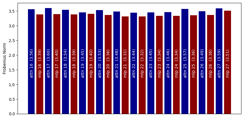
We see that, in general, the SONAR maps tend to put more emphasis on the Attention layers over the MLP layers. The difference is noticeable but not huge (3.56 Attention vs 3.39 MLP in layer 16). 

I suspect having better weight decay or something similar would probably result in more fine-grained predictions, or possibly there are better metrics than just Frobenius norm.

 

Quality of Scoring - Correlational Analysis

To what degree are the different Residual Stream Decoders, SONAR ParaScope and Continuation ParaScope, correlated or uncorrelated at getting the right answer? There are various correlation metrics like Pearson, Spearman and Kendall-Tau, which have their uses, but they mostly gave similar results, but I show Kendall Correlation below.

How correlated is the same score for different methods?

The simplest "score" we can correlate things between, is to compare lengths of generation. We also compare against scoring along "subject match". We note that for the methods that are any good, the lengths are quite correlated. This at least shows things are OK.

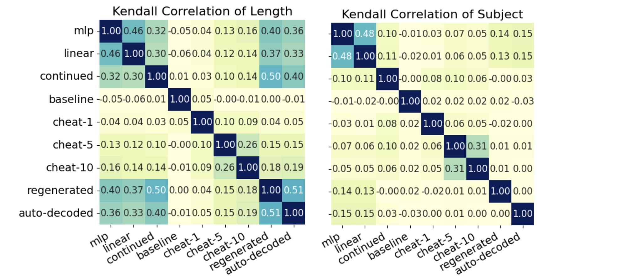
We can generally see that the MLP and Linear residual-to-sonar maps have very correlated scoring, more-so than most other methods between each other. For other scoring metrics, such as subject match, the correlation is much less. MLP and Linear maps seem to have high correlation, but other methods not so much. In particular, regenerated and auto-decoded have low correlation, likely because they both score almost perfectly almost all the time.

 

How correlated are different scores for the same method?

We also check if the different scores are capturing different things, and if there are correlated failures that do not exist in the data. 

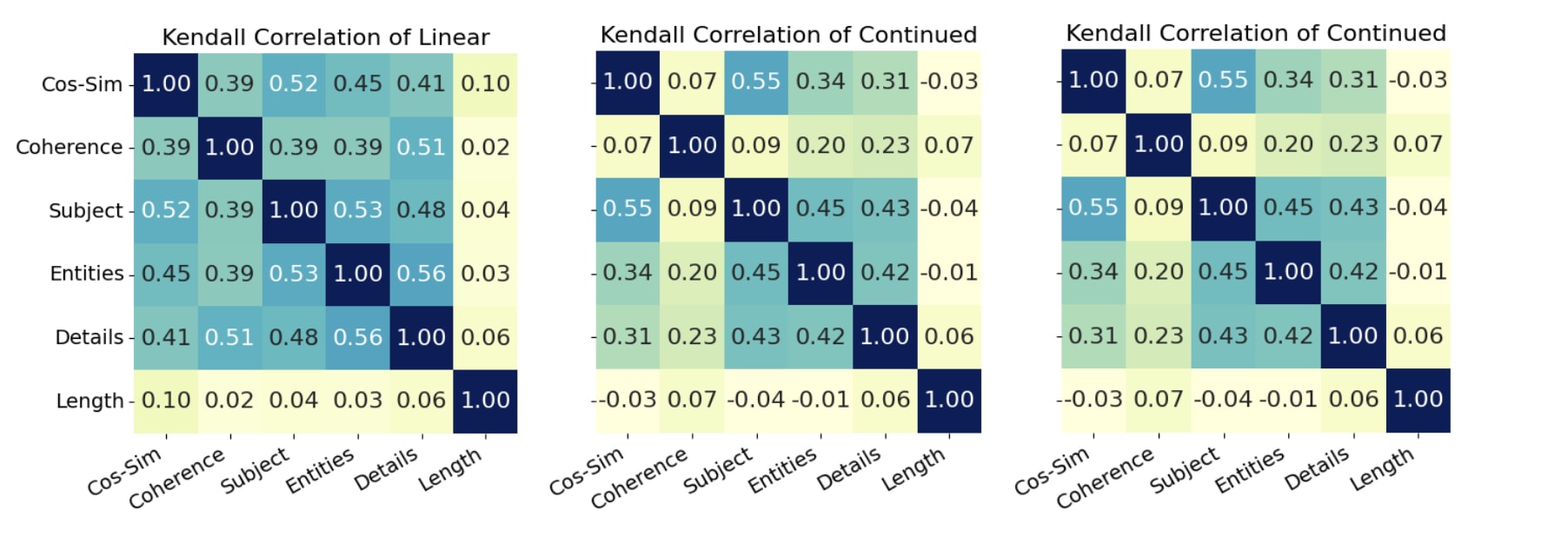
It seems like, overall, Linear seems to have higher inter-score correlations, likely because there are more cases where the output is completely incoherent, and thus, all the scores drop together. The scoring correlation seems similar-ish between Continuation ParaScope and the Regenerated baseline. 

 

To me, these results seem to show that the Continuation ParaScope and SONAR ParaScope seem to work pretty independently of each-other, and we also see that the SONAR ParaScopes seem to mostly fail due to many incoherent outputs.

---

Discussion and Limitations

Overall, we can see there is clear evidence that the model, Llama-3.2-3B-Instruct, is doing at least some "planning" for the immediately upcoming text, and this makes sense. The two Residual Stream Decoders that we propose: Continuation ParaScope and SONAR ParaScope, both seem to be able to sometimes, but not always, capture what the upcoming paragraph is likely to look like. 

The simplicity of these methods likely indicates that these are not likely to be over-fitting on the residual stream data, showing a proof of concept, and additional optimization seems like it would likely lead to far better Residual Stream Decoders. 

There is much work that could be done, both for immediate ParaScope Residual Stream Decoders, and for longer-horizon Residual Stream Decoders.

Potential future work on ParaScopes:

• It would make sense to try to understand why the SONAR ParaScopes often give incoherent outputs. It may be the case that the SONAR ParaScopes were not trained sufficiently well for handling noisy inputs, and some relatively simple fine-tuning may help with ensuring better decoding.
  • There is already some precedent with this in Meta's Large Concept Models paper. One could possibly use similar robustness training.
• Current SONAR ParaScope Maps have only been tested on residual stream diffs. It may be the case that summed residual streams, or intermediate activations such as MLP Neuron activations and attention pre-out activations may work better for the simple residual-to-sonar map.
• The current training for MLP and SONAR ParaScope maps were quite basic^[1], it might be that simple improvements to the training setup, such as using something better than MSE (e.g: SONAR Decoder CE Loss) would work better
• The Continuation ParaScope experiments were also relatively basic, simply replacing the residual stream of one token and running. While we did a couple of experiments in the Extracting Paragraphs paper, there are still possible improvements one could make, such as having a fine-tuned model that knows to better focus on the imported, or increasing the "intensity" of the activations.

• The scoring so far seems fine, and I like the Rubric scoring I have, but it could still be far improved. There may be better baselines for comparison.

   

Future work on broader Residual Stream Decoders:

• It would be better to understand whether the outputs are meerly correlational "implicit planning", or if there is also a degree of "explicit planning.
• I would like to expand the work to be able to handle understanding what longer-term outcomes the LLMs might be steering towards if possible.
  • Looking at "n+2" paragraphs seems like it would be relatively straight forward to test, but I don't have particular reason to think they would work that well.
  • I expect looking at final-state paragraphs may possibly lead to better probing results if done correctly, but how to do this well seems tricky
• Is it possible to gain useful information about various aspects of what the output looks like using these probes?
  • In particular, would it be possible to compare single aspects like "truth VS lie" after they have been mapped into the SONAR space?

Overall, I am hopeful that there are some interesting results to be had via the Residual Stream Decoders approach, which could be used for better testing and monitoring AI systems in the future.

If you think this work is interesting, and would like to learn more or potentially collaborate, feel free to reach out by messaging me on LessWrong or scheduling a short call.  

Acknowledgements 

 Thanks to my various collaborators: Eloise Benito-Rodriguez, Angelo Benoit, Lovkush Agarwal, Zainab Ali Majid, Lucile Ter-Minassian, Einar Urdshals [LW · GW], Jasmina Urdshals [LW · GW], Mikolaj

Appendix

1. ^{^}

   HyperParameters for SONAR Maps

   For the MLP and Linear SONAR Maps, I did a quick sweep over hyper-parameters with wandb. I found that using skipping the first half of layers (0-15) and only using the second half (layers 16 - 27) worked almost identically well as the full model, or slightly better, but trained a good bit faster. This is in line with the section above: "Which layers contribute the most?"

   Linear Model

   Normalize( 61,440 ) → 1,024

   Train on a batch size of 1,024. Use the last 50% of residual diff layer activations. The learning rate is set to 2e-5, learning rate decay of 0.8 per epoch for 10 epochs. Weight decay of 1e-7 also applied. Achieved a training loss of 0.750 and validation loss of 0.784. 

   MLP Model

   Normalize( 61,440 ) → GeLU( 8,192 ) → GeLU( 8,192 ) → 1,024

   Train on a batch size of 1,024 with two MLP hidden layers of dimension 8,192. . The learning rate is set to 2e-5, with a decay of 0.8 per epoch over 10 epochs. A higher weight decay of 2e-5 a dropout of 0.05 is applied for regularization. The model achieved a training loss of 0.724 and a validation loss of 0.758, showing consistent performance with slight overfitting.

2. ^{^}

   ParaScope Output Comparisons

   Original	Black seed oil is a rich source of essential fatty acids, particularly oleic acid, linoleic acid, and alpha-linolenic acid. The oil is also a good source of vitamins, minerals, and antioxidants. Accor...
   Linear	Black pepper oil mixture is a nutrient rich oil of black pepper and acetaldehyde, which contains an average of 50 grams of vitamin A. The black pepper oil mixture is characterized by oil richness and...

   Original	* **Rocketman Sing-A-Long** - July 12th at 7pm and 9pm at Regal Cinemas and AMC Theatres Join us for a special sing-along screening of the critically-acclaimed biopic Rocketman, starring Taron Egerton
   Auto-decoded:	* "Rockin' Man" 12:00pm - 10:30pm * * * * * * * * * * * * * * * * * * * * * * * * * * * * * * * * * * * * * * * * * * * * * * * * * * * * * * * * * * * * * * * * * * * * * * * * * * * * * * * * * * *

   Original:	According to Cawley, the outage was caused by a combination of factors, including worn-out equipment and a power surge that affected multiple substations in the area. "Our team worked diligently to re...
   Auto-decoded:	According to Cawley, the failure was the result of a combination of equipment, including obsolete equipment and overloading of the area with multiple power stations. "Our team worked diligently to con...

   Original:	At just 21 years old, Sigrid Lid Æ Pain, known professionally as Sigrid, has already made a significant impact on the music industry. The Norwegian pop sensation's rise to fame has been nothing short...
   Auto-decoded:	With only 21 years old, Sigrid Liddig Seer, known professionally as Sigrid, has already had a significant impact on the music industry. The rise of the Norwegian pop sensation has been nothing short o...

   I don't want to clutter the post by adding a bunch of examples here, so see the GitHub for more.

3. ^{^}

   BLEU and ROGUE scores

   Here are the BLEU or ROUGE scores or similar, but the task here is not really translation, and I want to have more room for fuzzy scoring, so I didn't think it would be super relevant here. Regardless, these are considered standard so I include them.

   Method	SacreBLEU Mean ± StDev	ROGUE-1 F1 Score	ROUGE-2 Precision	ROUGE-L F1 Score
   mlp	2.92 ± 2.81	0.27 ± 0.12	0.07 ± 0.07	0.19 ± 0.08
   linear	2.81 ± 2.82	0.27 ± 0.12	0.07 ± 0.07	0.19 ± 0.08
   continued	4.42 ± 4.92	0.27 ± 0.10	0.06 ± 0.07	0.18 ± 0.07
   baseline	0.60 ± 0.67	0.10 ± 0.08	0.01 ± 0.02	0.07 ± 0.06
   cheat-1	1.41 ± 1.53	0.16 ± 0.08	0.02 ± 0.04	0.12 ± 0.06
   cheat-5	7.58 ± 5.35	0.29 ± 0.09	0.14 ± 0.14	0.23 ± 0.07
   cheat-10	15.91 ± 8.57	0.38 ± 0.10	0.25 ± 0.15	0.32 ± 0.09
   regenerated	22.65 ± 19.64	0.50 ± 0.17	0.28 ± 0.21	0.38 ± 0.18
   auto-decoded	58.27 ± 24.32	0.81 ± 0.18	0.69 ± 0.21	0.78 ± 0.20

0 comments

Comments sorted by top scores.