How To Think About Overparameterized Models

post by johnswentworth · 2021-03-03T22:29:13.126Z · LW · GW · 4 comments

Contents

  Ridges, Not Peaks
  Priors and Sampling, Not Likelihoods and Estimation
  Example: Overparameterized Linear Regression
    Traditional-Style Regression
    (Slightly) Overparameterized Regression
    (Very) Overparameterized Regression
None
4 comments

So, you’ve heard that modern neural networks have vastly more parameters than they need to perfectly fit all of the data. They’re operating way out in the regime where, traditionally, we would have expected drastic overfit, yet they seem to basically work. Clearly, our stats-101 mental models no longer apply here. What’s going on, and how should we picture it?

Maybe you’ve heard about some papers on the topic, but didn’t look into it in much depth, and you still don’t really have an intuition for what’s going on. This post is for you. We’ll go over my current mental models for what’s-going-on in overparameterized models (i.e. modern neural nets).

Disclaimer: I am much more an expert in probability (and applied math more generally) than in deep learning specifically. If there are mistakes in here, hopefully someone will bring it up in the comments.

Assumed background knowledge: multi-dimensional Taylor expansions, linear algebra.

Ridges, Not Peaks

First things first: when optimizing ML models, we usually have some objective function where perfectly predicting every point in the training set yields the best possible score. In overparameterized models, we have enough parameters that training indeed converges to zero error, i.e. all data points in the training set are matched perfectly.

Let’s pick one particular prediction setup to think about, so we can stick some equations on this. We have a bunch of $(x,y)$ data points, and we want to predict $y$ given $x$. Our ML model has some parameters $\theta$, and its prediction on a point $x^{\left(n\right)}$ is $f(x^{\left(n\right)},\theta )$. In order to perfectly predict every data point in the training set, $\theta$ must satisfy the equations

$\forall n:y^{\left(n\right)}=f(x^{\left(n\right)},\theta )$

Assuming $y^{\left(n\right)}$ is one-dimensional (i.e. just a number), and we have $N$ data points, this gives us $N$ equations. If $\theta$ is $k$-dimensional, then we have $N$ equations with $k$ variables. If the number of variables is much larger than the number of equations (i.e. $k>>N$, parameter-dimension much greater than number of data points), then this system of equations will typically have many solutions.

In fact, assuming there are any solutions at all, we can prove there are infinitely many - an entire high-dimensional surface of solutions in $\theta$-space. Proof: let ${\theta }^{\ast }$ be a solution. If we make a small change $d{\theta }^{\ast }$, then $f(x^{\left(n\right)},\theta )$ changes by ${\nabla }_{\theta }f(x^{\left(n\right)},{\theta }^{\ast })\cdot d{\theta }^{\ast }$. For all the equations to remain satisfied, after shifting ${\theta }^{\ast }\to {\theta }^{\ast }+d{\theta }^{\ast }$, these changes must all be zero:

$\forall n:0={\nabla }_{\theta }f(x^{\left(n\right)},{\theta }^{\ast })\cdot d{\theta }^{\ast }$

Key thing to notice: this is a set of linear equations. There are still $N$ equations and still $k$ variables (this time $d{\theta }^{\ast }$ rather than $\theta$), and since they’re linear, there are guaranteed to be at least $k-N$ independent directions along which we can vary $d{\theta }^{\ast }$ while still solving the equations (i.e. the right nullspace of the matrix ${\nabla }_{\theta }f(x^{\left(n\right)},{\theta }^{\ast })$ has dimension at least $k-N$). These directions point exactly along the local surface on which the equations are solved.

Takeaway: we have an entire surface of dimension (at least) $k-N$, sitting in the $k$-dimensional $\theta$-space, on which all points in the training data are predicted perfectly.

What does this tell us about the shape of the objective function more generally?

Well, we have this (at least) $k-N$ dimensional surface on which the objective function achieves its best possible value. Everywhere else, it will be lower. The “global optimum” is not a point at the top of a single peak, but rather a surface at the high point of an entire high-dimensional ridge. So: picture ridges, not peaks.

Before we move on, two minor comments on generalizing this model.

• “Predict $y$ given $x$” is not the only setup deep learning is used for; we also have things like “predict/generate/compress samples of $x$” or RL. My understanding is that generally-similar considerations apply, though of course the equations will be different.
• If $y$ is more than one-dimensional, e.g. dimension $d$, then the perfect-prediction surface will have dimension at least $k-Nd$ rather than $k-N$.

Priors and Sampling, Not Likelihoods and Estimation

So there’s an entire surface of optimal points. Obvious next question: if all of these points are optimal, what determines which one we pick? Short answer: mainly initial parameter values, which are typically randomly generated.

Conceptually, we randomly sample trained parameter values from the perfect-prediction surface. To do that, we first sample some random initial parameter values, and then we train them - roughly speaking, we gradient-descend our way to whatever point on the perfect-prediction surface is closest to our initial values. The key problem is to figure out what distribution of final (trained) parameter values results from the initial distribution of parameter values.

One key empirical result: during training, the parameters in large overparameterized models tend to change by only a small amount. (There’s a great visual of this in this post. It’s an animation showing weights changing over the course of training; for the larger nets, they don’t visibly change at all.) In particular, this means that linear/quadratic approximations (i.e. Taylor expansions) should work very well.

For our purposes, we don’t even care about the details of the ridge-shape. The only piece which matters is that, as long as we’re close enough for quadratic approximations around the ridge to work well, the gradient will be perpendicular to the directions along which the ridge runs. So, gradient descent will take us from the initial point, to whatever point on the perfect-prediction surface is closest (under ordinary Euclidean distance) to the initial point.

Stochastic gradient descent (as opposed to pure gradient descent) will contribute some noise - i.e. diffusion along the ridge-direction - but it should average out to roughly the same thing.

From there, figuring out the distribution from which we effectively sample our trained parameter values is conceptually straightforward. For each point ${\theta }^{\ast }$ on the perfect-prediction surface, add up the probability density of the initial parameter distribution at all the points which are closer to ${\theta }^{\ast }$ than to any other point on the perfect-prediction surface.

We can break this up into two factors:

• How large a volume of space is closest to ${\theta }^{\ast }$? This will depend mainly on the local curvature of the perfect-prediction-surface (higher where curvature is lower)
• What’s the average density of the initial-parameter distribution in that volume of space?

Now for the really hand-wavy approximations:

• Let’s just ignore that first factor. Assume that the local curvature of the perfect-prediction surface doesn’t change too much over the surface, and approximate it by a constant. (Everything’s on a log-scale, so this is reasonable unless the curvature changes by many orders of magnitude.)
• For the second factor, let’s assume the average density of the initial-parameter distribution over the volume is roughly proportional to the density at ${\theta }^{\ast }$. (This is hopefully reasonable, since we already know initial points are quite close to final points in practice.)

Are these approximations reasonable? I haven’t seen anyone check directly, but they are the approximations needed in order for the results in e.g. Mingard et al [LW · GW] to hold robustly, and those results do seem to hold empirically.

The upshot: we have an effective “prior” (i.e. the distribution from which the initial parameter values are sampled) and “posterior” (i.e. the distribution of final parameter values on the perfect-prediction surface). The posterior density is directly proportional to the prior density, but restricted to the perfect-prediction surface. This is exactly what Bayes’ rule says, if we start with a distribution $P\left[\theta \right]$ and then update on data of the form “$\forall n:y^{\left(n\right)}=f(x^{\left(n\right)},\theta )$”. Our posterior is then $P[\theta |\forall n:y^{\left(n\right)}=f(x^{\left(n\right)},\theta \left)\right]$, and our final parameter-values are a sample from that distribution.

Note how this differs from traditional statistical practice. Traditionally, we maximize likelihood, and that produces a unique “estimate” of $\theta$. While today’s ML models may look like that at first glance, they’re really performing a Bayesian update of the parameter-value-distribution, and then sampling from the posterior.

Example: Overparameterized Linear Regression

As an example, let’s run a plain old linear regression. We’ll use an overparameterized model which is equivalent to a traditional linear regression model, in order to make the relationship clear.

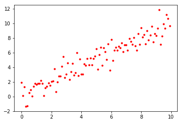
We have 100 $(x,y)$ pairs, which look like this:

I generated these with a “true” slope of 1, i.e. $y=1\ast x+noise$, with standard normal noise.

Traditional-Style Regression

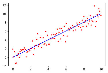
We have one parameter, $c$, and we fit a model $y^{\left(n\right)}=c{x}^{\left(n\right)}+{\xi }^{\left(n\right)}$, with standard normal-distributed noise ${\xi }^{\left(n\right)}$. This gives log likelihood

$logP\left[y|a\right]=-\frac{1}{2}{\sum }_n(y^{\left(n\right)}-c{x}^{\left(n\right)}{)}^2$

… plus some constants. We choose $c^{\ast }$ to maximize this log-likelihood. In this case, $c^{\ast }=1.010$, so the line looks like this:

(Slightly) Overparameterized Regression

We use the exact same model, $y^{\left(n\right)}=c{x}^{\left(n\right)}+{\xi }^{\left(n\right)}$, but now we explicitly consider the ${\xi }^{\left(n\right)}$ terms “parameters”. Now our parameters are $(c,{\xi }^{\left(1\right)},\dots ,{\xi }^{\left(N\right)})$, and we’ll initialize them all as samples from a standard normal distribution (so our “prior” on the noise terms is the same distribution assumed in the previous regression). We then optimize $(c,{\xi }^{\left(1\right)},\dots ,{\xi }^{\left(N\right)})$ to minimize the sum-of-squared-errors

$\frac{1}{2}{\sum }_n(y^{\left(n\right)}-c{x}^{\left(n\right)}-{\xi }^{\left(n\right)}{)}^2$

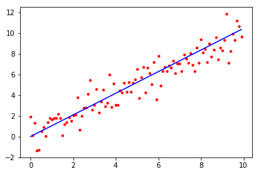
This ends up approximately the same as a Bayesian update on $\forall n:y^{\left(n\right)}=c{x}^{\left(n\right)}-{\xi }^{\left(n\right)}$, and our final $c$-value 1.046 is not an estimate, but rather a sample from the posterior. Although the “error” in our $c$-posterior-sample here is larger than the “error” in our $c$-estimate from the previous regression, the implied line is visually identical:

Note that our model here is only slightly overparameterized; $k=N+1$, so the perfect prediction surface is one-dimensional. Indeed, the perfect prediction surface is a straight line in $(c,{\xi }^{\left(1\right)},\dots ,{\xi }^{\left(N\right)})$ - space, given by the equations $y^{\left(n\right)}=c{x}^{\left(n\right)}+{\xi }^{\left(n\right)}$.

(Very) Overparameterized Regression

Usually, we say that the noise terms are normal because they’re a sum of many small independent noise sources. To make a very overparameterized model, let’s make those small independent noise sources explicit: $y^{\left(n\right)}=c{x}^{\left(n\right)}+\sqrt{\frac{3}{N}}{\sum }_{i=0}^{100}{\xi }_i^{\left(n\right)}$. Our parameters are $c$ and the whole 2D array of $\xi$’s, with standard normal initialization on $c$, and Uniform(-1, 1) initialization on $\xi$. (The $\sqrt{\frac{3}{N}}$ is there to make the standard deviation equivalent to the original model.) As before, we minimize sum-of-squared-errors.

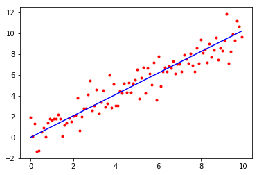
This time our $c$-value is 1.031. The line still looks exactly the same. This time, we’re much more overparameterized - we have $k=100N+1$, so the perfect prediction surface has dimension $99N+1$. But conceptually, it still works basically the same as the previous example.

Code for all these is here.

In all these examples, the underlying probabilistic models are (approximately) identical. The latter two (approximately) sample from the posterior, rather than calculating a maximum-log-likelihood parameter estimate, but as long as the posterior for the slope parameter is very pointy, the result is nearly the same. The main difference is just what we call a "parameter" and optimize over, rather than integrating out.

4 comments

Comments sorted by top scores.