Degeneracies are sticky for SGD
post by Guillaume Corlouer (Tancrede), Nicolas Macé (NicolasMace) · 2024-06-16T21:19:53.362Z · LW · GW · 1 commentsContents
  Introduction
      Main takeaways
  Terminology and notation
  Background and some related work
    Geometry of the loss landscape in deep learning
    Diffusion theory of SGD
    Singular learning theory
    Developmental interpretability
  Results
    Models
    SGD can cross a potential barrier from a sharp minimum
    SGD converges toward the most degenerate point along a degenerate line in a 2D potential
    SGD get stuck along degenerate directions
    The sharpness of the non degenerate minimum and the learning rate mostly affect SGD escape
  Connection between degeneracies and SGD dynamics
  Discussion
    Takeaways
    Limitations
    Future work
  Acknowledgments
  Appendix: Hessian and SGD noise covariance are proportional around critical points of linear models
    Hessian of the potential
    SGD noise covariance
None
1 comment
Introduction
Singular learning theory (SLT) is a theory of learning dynamics in Bayesian statistical models. It has been argued that SLT could provide insights into the training dynamics of deep neural networks. However, a theory of deep learning inspired by SLT is still lacking. In particular it seems important to have a better understanding of the relevance of SLT insights to stochastic gradient descent (SGD) – the paradigmatic deep learning optimization algorithm.
We explore how the degeneracies[1] of toy, low dimensional loss landscapes affect the dynamics of stochastic gradient descent (SGD).[2] We also investigate the hypothesis that the set of parameters selected by SGD after a large number of gradient steps on a degenerate landscape is distributed like the Bayesian posterior at low temperature (i.e., in the large sample limit). We do so by running SGD on 1D and 2D loss landscapes with minima of varying degrees of degeneracy.
While researchers experienced with SLT are aware of differences between SGD and Bayesian inference, we want to understand the influence of degeneracies on SGD with more precision and have specific examples where SGD dynamics and Bayesian inference can differ.
Main takeaways
- Degeneracies influence SGD dynamics in two ways: (1) Convergence to a critical point is slower, the more degenerate the critical point is; (2) On a (partially) degenerate manifold, SGD preferentially escapes along non-degenerate directions. If all directions are degenerate, then we empirically observe that SGD is "stuck"
- To explain our observations, we show that, for our models, SGD noise covariance is proportional to the Hessian in the neighborhood of a critical point of the loss
- Thus SGD noise covariance goes faster to zero along more degenerate directions, to leading order in the neighborhood of a critical point
- Qualitatively we observe that the concentration of the end-of-training distribution of parameters sampled from a set of SGD trajectories sometimes differ from the Bayesian posterior as predicted by SLT because of:
- The hyperparameters such as the learning rate
- The number of orthogonal degenerate directions
- The degree of degeneracy in the neighborhood of a minimum
Terminology and notation
We advise the reader to skip this section and come back to it if notation or terminology is confusing.
Consider a sequence of input-output pairs . We can think of as input data to a deep learning model (e.g., a picture, or a token) and as an output that model is trying to learn (e.g., whether the picture represents a cat or a dog, or a what the next token is). A deep learning model may be represented as a function , where is a point in a parameter space . The one-sample loss function, noted (), is a measure of how good the model parametrized by is a predicting the output on input . The empirical loss over samples is noted . Noting the probability density function of input-output pairs, the theoretical loss (or the potential) writes .[4] The loss landscape is the manifold associated with the theoretical loss function .
A point is a critical point if the gradient of the theoretical loss is at i.e. . A critical point is degenerate if the Hessian of the loss has at least one eigenvalue at . An eigenvector of with zero eigenvalue is a degenerate direction.
The local learning coefficient measures the greatest amount of degeneracy of a model around a critical point . For the purpose of this work, if locally then the local learning coefficient is given by . We say that a critical point is more degenerate than a critical point if . Intuitively this means that the flat basin is broader around than around .[5] See figures [LW · GW] in the experiment section for visualizations of degenerate loss landscape with different degrees of degeneracies.
SGD and its variants with momentum are the optimization algorithms behind deep learning. At every time step , one samples a batch of datapoints from a dataset of samples, uniformly at random without replacement. The parameter update of the model satisfies:
where is called the SGD noise. It has zero mean and covariance matrix .[6] SGD is the combination of a drift term and a noise term .
While SGD and Bayesian inference are fundamentally different learning algorithms, we can compare the distribution of SGD trajectories after updates of SGD with the Bayesian posterior after updating on batches according to Bayes' rule and where each is a batch drawn at time . For SGD, random initialization plays the role of the prior , while the loss over the batches plays the role of the negative log-likelihood over the dataset . Under some (restrictive) assumptions Mandt et al (2017) demonstrate an approximate correspondence between Bayesian inference and SGD. In this post, we are particularly interested in understanding in more details the influence of degenerate minima on SGD and the difference between the Bayesian posterior and SGD when the assumption that critical points are non-degenerate no longer holds.
Background and some related work
Geometry of the loss landscape in deep learning
SGD is an optimization algorithm updating parameters over a loss-landscape which is a highly non-convex, non-linear, and high-dimensional manifold. Typically, around critical point of the loss-landscape, the distribution of eigenvalues of the empirical Hessian of a deep neural network peaks around zero, with a long tail of large positive eigenvalues and a short negative tail of negative eigenvalues. In other words, critical points of the loss landscape of large neural networks tend to be saddle points with many flat plateaus, a few negatively curved directions along which SGD can escape and positively curved directions going upward. A range of empirical studies have observed that SGD favors flat basins. Flatness is associated with better generalization properties for a given test loss.
Diffusion theory of SGD
Approximating SGD by a Langevin dynamics – where SGD noise is approximated by Gaussian white noise – and assuming the noise to be isotropic and the loss to be quadratic around a critical point of interest, SGD approximates Bayesian inference. However the continuity, isotropicity and regularity assumptions tend to be violated in deep learning. For example, at degenerate critical points, it has been empirically observed that SGD noise covariance is proportional to the Hessian of the loss, leading to noise anisotropy that depends on the eigenvalues of the Hessian. Quantitative analyses have suggested that this Hessian-dependent noise anisotropy allows SGD to find flat minima exponentially faster than the isotropic noise associated with Langevin dynamics in Gradient Descent (GD), and that the anisotropy of SGD noise induces an effective regularization favoring flat solutions.
Singular learning theory
Singular learning theory [? · GW] (SLT) shows that, in the limit of infinite data, minimizing the Bayesian free energy [? · GW] of a statistical model around a critical point is approximately determined by a tradeoff between the log-likelihood (model fit) and the local learning coefficient [? · GW], i.e. the local learning coefficient is a well defined notion of model complexity [LW · GW] for the Bayesian selection of degenerate models. In particular, within a subspace of constant loss, SLT shows that the Bayesian posterior will most concentrate around the most degenerate minimum. A central result of SLT is that, for minima with the same loss, a model with lower learning coefficient has a lower Bayesian generalization error (Watanabe 2022, Eq. 76).
Intuitively, the learning coefficient is a measure of "basin broadness". Indeed it corresponds to the smallest scaling exponent of the volume [? · GW] of the loss-landscape around a degenerate critical point . More specifically, defining the volume as the measure of the set then there exist a unique and such that
Thus to leading order near a critical point, the learning coefficient is the volume scaling exponent.
Developmental interpretability
Singular learning theory has already shown promising applications for understanding the training dynamics of deep neural networks. Developmental interpretability [? · GW] aims to understand the stage-wise development of internal representations and circuits during the training of deep learning models. Notable recent results:
- In a toy model of superposition, the learning coefficient helps to determine structural change in the geometry of features represented in superposition during training.
- Plateaus in the local learning coefficient mark boundaries between the stagewise development of in-context learning and in-context linear regression during the training dynamics of a two-layer transformer.
Results
We investigate SGD on 1D and 2D degenerate loss-landscape from statistical models that are linear in data and non-linear in parameters.
- In one dimension, we study the escape dynamics from a non-degenerate to a degenerate minimum, as well as the dynamics from a degenerate to a more degenerate minimum. Depending on the value of the learning rate and the sharpness of a non-degenerate minimum (locally quadratic), we observe that either:
- All SGD trajectories escape at a constant rate from a non-degenerate to a degenerate minimum across a potential barrier, in line with SLT expectations for the Bayesian posterior; or
- When both basins are degenerate, with different degrees of degeneracies, no SGD trajectory escape during our simulations.
- In two dimensions, we study a loss landscape where a 1d degenerate line (a "valley") is connected to a fully degenerate point. SLT expects that, as more data is seen, the posterior is first spread out in the valley, and then concentrates on the most degenerate point.
- If the valley has a non-degenerate direction, SGD "uses it" to converge to the fully degenerate point. Qualitatively, the behaviour of the distribution of SGD trajectories after a large enough number of SGD steps resembles the Bayesian posterior.
- However, when all independent directions spanning the valley are degenerate, SGD does not necessarily converge to the most degenerate minima and appears to get stuck on a minimum of intermediate degeneracy.
- In 2D we can see more clearly that degenerate directions are sticky for SGD with SGD noise being lower along degenerate directions and trajectories getting stuck on a degenerate line, even though there is no potential barrier
Models
We consider models of the form where is a polynomial. In practice, we take or , i.e. one- or two-dimensional models.
We train our models to learn a linear relationship between input and output data.
That is, a given model is trained on data tuples with , where is a normally distributed noise term, i.e. . We also choose . For the sake of simplicity, we'll set henceforth.[7] The empirical loss on a given batch of size at time is given by:
Taking the expectation of the empirical loss over the data with true distribution , the potential (or theoretical loss) writes l, up to a positive affine transformation that we'll omit as it does not affect loss-minimization. We study the SGD dynamics on such models.
First we will investigate cases (in 1D and 2D) where SGD converges to the most degenerate minimum, which is consistent with SLT's predictions of the dynamics of the Bayesian posterior. Then, we will investigate potentials where SGD does not and instead gets stuck in a degenerate region that is not necessarily the most degenerate.
SGD can cross a potential barrier from a sharp minimum
In one dimension, we study models whose potential is given by:
This potential can be derived from the empirical loss with a statistical model and with . While such a model is idiosyncratic, it presents the advantages of being among the simplest models with two minima. In this section, we set and . Thus, the minimum at is non-degenerate and the minimum at is degenerate. We observe that for a sufficiently large learning rate , SGD trajectories escape from the non-degenerate minimum to the degenerate one.
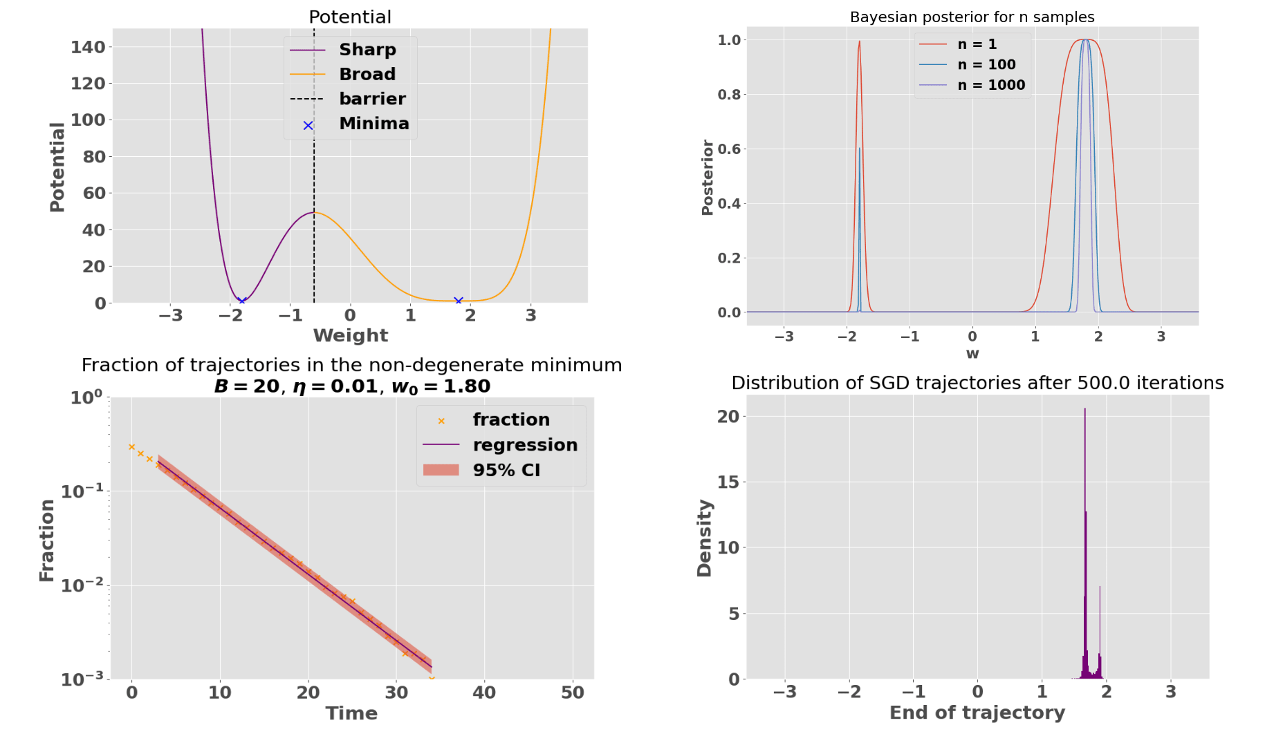
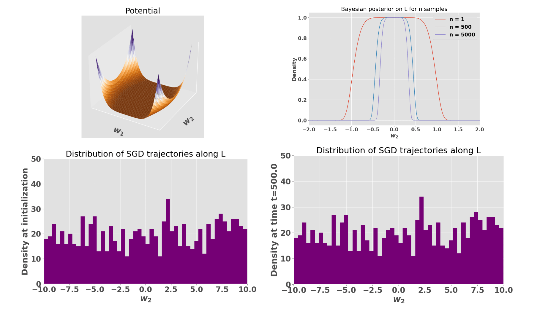
For instance, Fig. 1 above shows SGD trajectories initialized uniformly at random between and updated for for SGD iterations. Pretty quickly, almost all trajectories escape from the non-degenerate mininum to the degenerate minimum. Interestingly, the fraction of trajectories present in the regular basin exponentially decay with time.[8] Under such conditions, the qualitative behavior of the distribution of SGD trajectories is consistent with SLT predicting that the Bayesian posterior will most concentrate around the most degenerate minimum. However the precise forms of the posterior and the distribution of SGD trajectories differ in finite time (compare Fig. 1 upper right and Fig. 1 lower right).
SGD converges toward the most degenerate point along a degenerate line in a 2D potential
We investigate the dynamics of SGD on a 2D degenerate potential:
This potential has a degenerate minimum at the origin and a degenerate line defined by . In a neighborhood of the line that's not near the origin , we have . Thus, the potential is degenerate along but non-degenerate along . In a neighborhood of on the other hand, the potential is degenerate along both and . Thus, Bayesian posterior will (as a function of the number of observations made, starting from a diffuse prior) first accumulate on the degenerate line , and eventually concentrate at , since its degeneracy is higher.
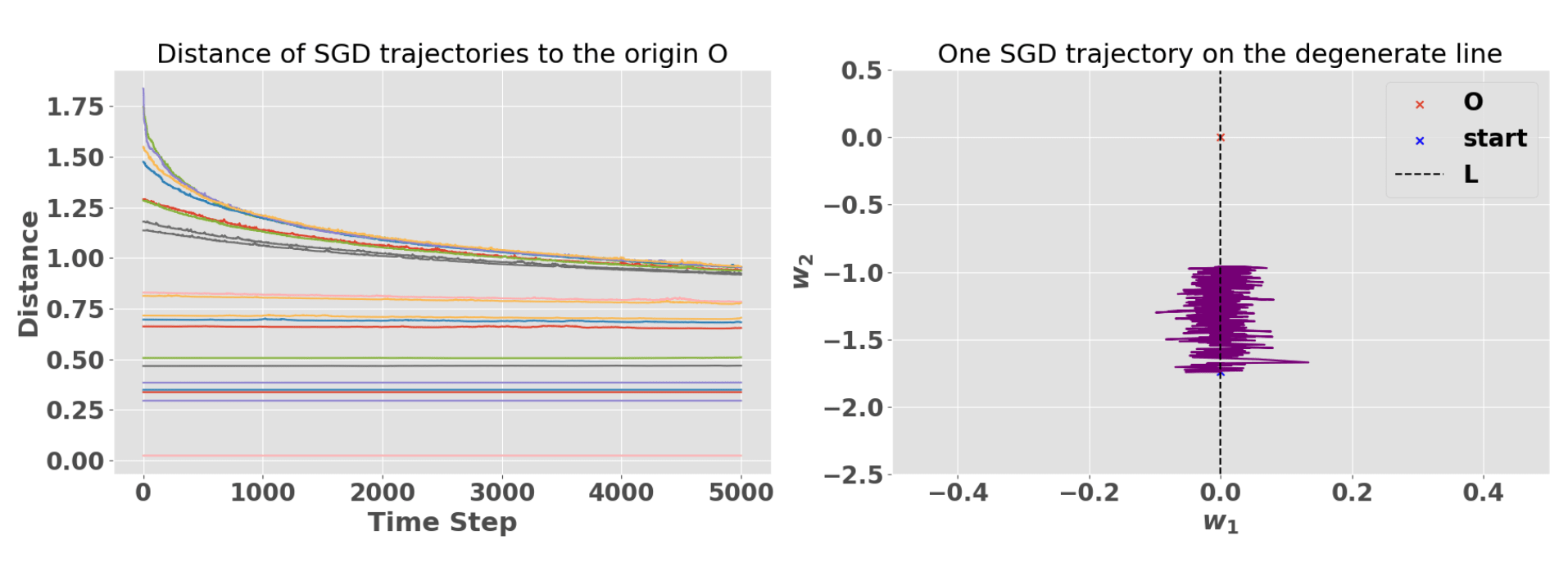
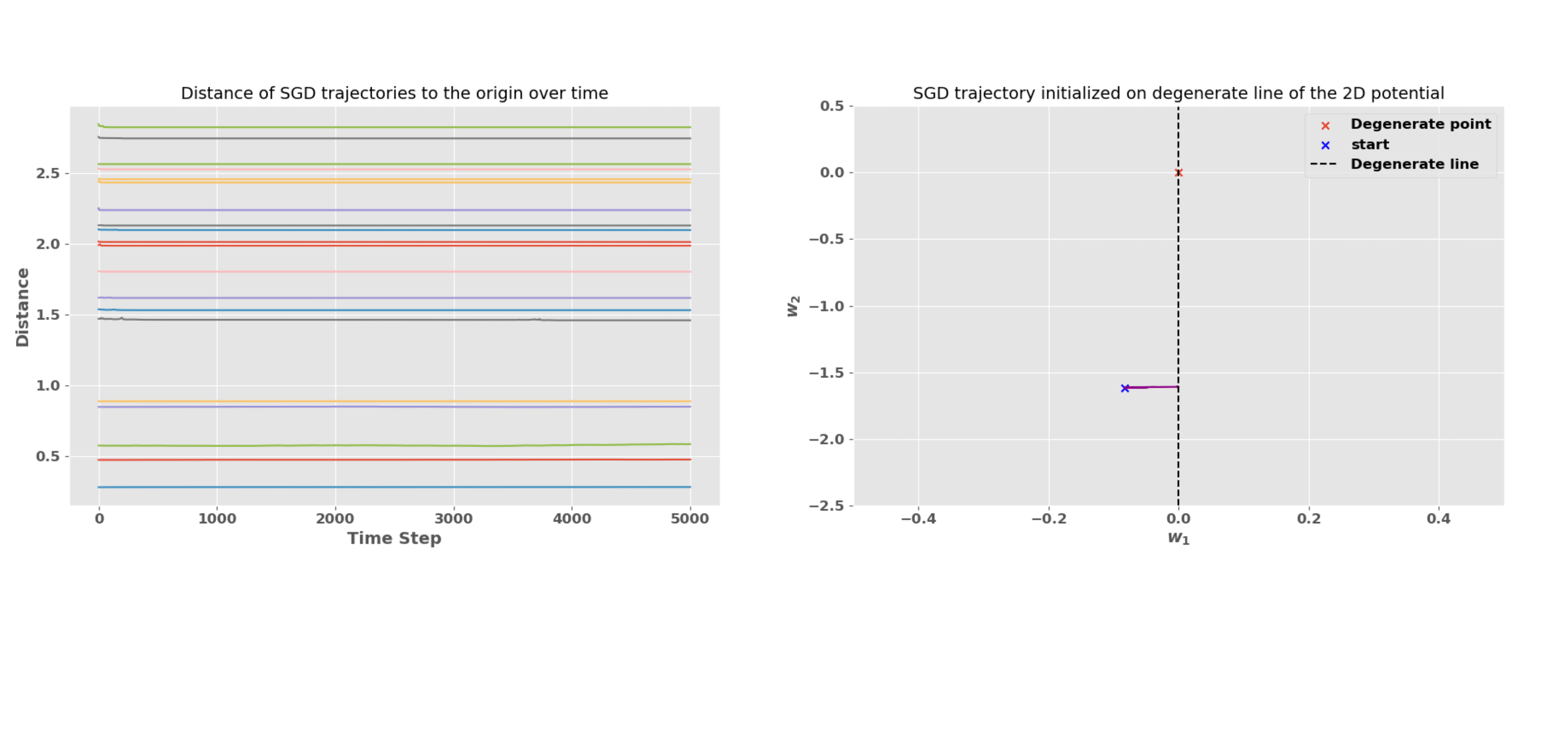
Naively, one might guess that points on the line are stable attractors of the SGD dynamics, since contains local minima and has zero theoretical gradient. However, SGD trajectories do not in fact get stuck on the line, but instead converge to the most degenerate point , in line with SLT predictions regarding the Bayesian posterior. This is because at any point on , finite batches generate SGD noise in the non-degenerate direction, pushing the system away from . Once no longer on , the system has a non-zero gradient along that pushes it towards the origin. This "zigzag" dynamics is shown on Fig. 3 right panel. Thus, the existence of non-degenerate directions seems crucial for SGD not to "get stuck". And indeed, in the next section we'll see that SGD can get stuck when this is not longer the case.
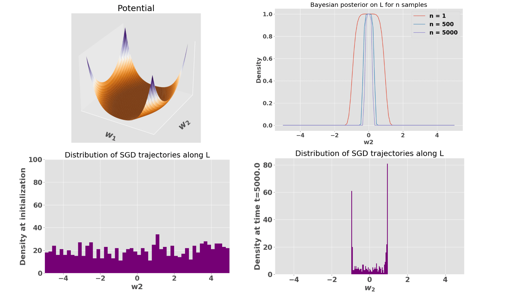
Fig. 2 (right) shows that the distribution of SGD trajectories along the degenerate line does no coincide with the Bayesian posterior. In the infinite time limit however, we conjecture that both the SGD and the Bayesian posterior distribution coincide and are Dirac distributions centered on . We can see the the trajectories being slowed down substantially as they approach the most degenerate minimum in the next figure.
SGD get stuck along degenerate directions
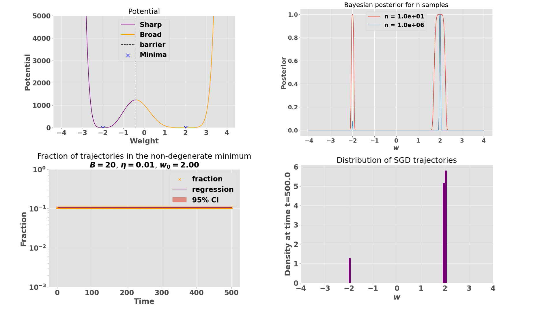
We now explore cases where SGD can get stuck. As we briefly touched on above [LW · GW], we conjecture that SGD diffuses away from degenerate manifolds along the non-degenerate directions, if they exist. Thus, we expect SGD to be stuck on fully degenerate ones (i.e., one such that all directions are singular). We first explore SGD convergence on the degenerate 1D potential:
The most degenerate minimum is while the least degenerate minimum is . In the large sample limit, SLT predicts that the Bayesian posterior concentrates around the most degenerate critical point . However, we observe that SGD trajectories initialized in the basin of attraction of get stuck around the least degenerate minimum and never escape to the most degenerate minimum . In theory, SGD would escape if it sees enough consecutive gradient updates to push it over the potential barrier. Such events are however unlikely enough that we couldn't observed them numerically. This result also holds when considering SGD with momentum.
We also compare the distribution of SGD trajectories with the Bayesian posterior for a given number of samples . Consistent with SLT predictions, the Bayesian posterior eventually concentrates completely around the most degenerate critical point, while SGD trajectories do not.[9]
In 2D, we investigate SGD convergence on the potential:
As above, the loss-landscape contains a degenerate line of equation . This time however, the line is degenerate along both directions. The loss and theoretical gradient are zero at each point of . The origin has a higher local learning coefficient (i.e., it is more degenerate) than minima on away from .
We examine the behavior of SGD trajectories. We observe that SGD does not converge to the most degenerate point . Instead, SGD appears to get stuck as it approaches the degenerate line . We also compare the distribution of SGD trajectories along the degenerate line with the non-normalized Bayesian posterior (upper right panel of Fig. 5). The Bayesian posterior concentrates progressively more around as the number of samples increase, while the distribution of SGD trajectories appears not to concentrate on , but instead to remain broadly distributed over the entire less degenerate line .
We can examine the stickiness effect of the degenerate line more closely by measuring the Euclidean distance of each SGD trajectory to the most degenerate point . We observe that this distance remains constant over time (see Fig. 6).
The sharpness of the non degenerate minimum and the learning rate mostly affect SGD escape
We explore the effect of hyperparameters on the escape rate of SGD trajectories. More specifically, we examine the impact of varying batch size , learning rate , and the sharpness (curvature) of the non degenerate minimum on the escape rate of SGD trajectories. We quantify the sharpness of the regular minimum indirectly by looking at the distance between the regular and degenerate minima. As this distance increases, the regular minimum minimum becomes sharper. Our observation indicate that the sharpness of the regular minimum and the learning rate have the strongest effect on the escape rate of SGD.
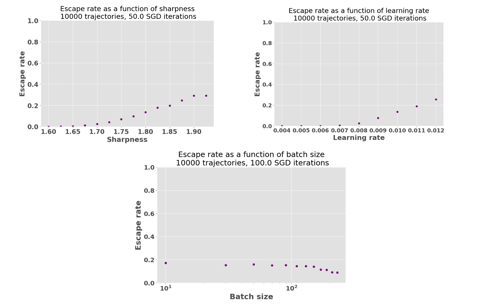
When the learning rate is above a certain threshold (approximately with the choice of parameters of Fig. 7) and the basin around the singular minimum is sufficiently sharp ( with parameters of Fig. 7), trajectories in the non-degenerate minimum can escape when a batch or a sequence of batches is drawn that makes the SGD noise term sufficiently large for the gradient to "push" the trajectory across the potential barrier. Under these conditions, the fraction of trajectories in the non degenerate minimum decrease exponentially with time until all trajectories escape toward the degenerate minimum.
Increasing the batch size decreases SGD noise, so intuitively, we should expect increasing batch size to decrease the escape rate of SGD trajectories. While we do observe a small effect of increasing the batch size on decreasing the escape rate it tends to be much less important compared to varying the sharpness and learning rate.[10]
Interestingly, and perhaps counterintuitively, in these experiments the difference between the sharpness of the non degenerate minimum matters more than the height of the potential barrier to cross. Indeed, while the barrier becomes higher, the non-degenerate minimum becomes sharper and easier for SGD to escape from.
Connection between degeneracies and SGD dynamics
Let's understand more carefully the influence of degeneracies on the convergence of SGD in our experiments. When the line is locally quadratic in , has a nonzero component along the horizontal direction for any . Therefore, the empirical gradient
also has a nonzero horizontal component. This prevents trajectories from getting stuck on the degenerate line until they reach the neighborhood of the origin. The Hessian of the potential also has a non-zero eigenvalue, meaning that the line isn't fully degenerate. This is no coincidence, as we'll shortly discuss.
However, when the model is quadratic in , the line of zero loss and zero theoretical gradient is degenerate in both the horizontal and vertical directions. In this case, and thus both the empirical and theoretical gradient vanish along the degenerate line, causing SGD trajectories to get stuck. This demonstrates a scenario where SGD dynamics contrast with SLT predictions about the Bayesian posterior accumulating around the most singular point. In theory, SGD trajectories slightly away from might eventually escape toward but in practice, with a large but finite number of gradient updates, this seems unlikely.
Generic case: In general, a relationship between the SGD noise covariance and the Hessian of the loss explains why SGD can get stuck along degenerate directions. In the appendix [? · GW], we show that SGD noise covariance is proportional to the Hessian in the neighborhood of a critical point for models that are real analytic in parameters and linear in input data. Thus, the SGD noise has zero variance along degenerate directions, in the neighborhood of a critical point. That implies that SGD cannot move along those directions, i.e. that they are "sticky".
If on the other hand a direction is non-degenerate, there is in general non-zero SGD variance along that direction, meaning that SGD can use that direction to escape (to a more degenerate minimum). (Note that this proportionality relation also shows that SGD noise is anisotropic since SGD noise covariance depends on the degeneracies around a critical point).
Discussion
Takeaways
Our experiments provide a better intuition for how degeneracies influence the convergence of SGD. Namely, we show that they have a stickiness effect on parameters updates.
Essentially we observe that:
- At a critical point, degenerate directions are "sticky", while non-degenerate directions are not: SGD will escape along non-degenerate directions
- In the neighborhood of a critical point, the more degenerate the critical point, the slower the convergence of SGD toward that critical point
- Mathematically, we can explain [? · GW] these observations by showing that SGD noise covariance is proportional to the Hessian of the loss at a critical point
- This suggest a connection between generalization, SGD noise covariance, and degeneracies in the loss landscape
- When a critical point is degenerate in every direction, SGD appears to get stuck. In particular, in our 2D experiment, SGD gets stuck around a minimum that is not the most degenerate, even though there is no potential barrier to cross
- There is not always a qualitative correspondence between the Bayesian posterior and the distribution of parameters selected by SGD. Important differences arise from variables affecting SGD dynamics such as:
- Finite training time
- The degree of degenerate directions around a local minimum
- The amount of linearly independent degenerate directions
- The learning rate
Limitations
- We only worked on 1D and 2D toy models which are very remote from the high dimensional loss-landscape of neural networks
- However it offers the advantage of building intuition and studying the effect of degenerate directions in greater details
- Our models factor into a polynomial in the parameters and a linear function of the input data. However in deep learning, activation functions can also be nonlinear in data (e.g., ReLU)
- For more realistic non-analytic and non-linear models, the conditions under which the proportionality between the noise covariance of SGD and the Hessian are not precisely known (to the best of our knowledge) although it has been studied in the literature
- For example, it has been shown to hold with some assumptions that partly relied on numerical observations, and it is therefore plausible that our observations generalize
- We worked with i.i.d. synthetic gaussian data
- Modern large language models are not typically trained to convergence and critical points tend to be saddle points rather than local or global minima
Future work
- Examining the behavior of SGD around degeneracies in more realistic loss landscapes
- Investigating the relationship between SGD noise covariance matrix and the Hessian in more details.
- It looks promising to model SGD as a stochastic differential equation (SDE) and study the distribution of SGD trajectories with the corresponding dynamical probability distribution arising from solutions of the SDE
- For example, one could model SGD as a Langevin dynamics with anisotropic Gaussian noise covariance matrix and get as a solution of a Fokker-Planck equation
- However, Langevin dynamics requires a continuous approximation which might miss important properties of SGD. More complex SDE, such as the underdamped Langevin equation might be more adequate
- In particular, having a good model of the probability distribution of SGD trajectories and sampling from that distribution to probe the local geometry around a degenerate critical point looks like an interesting direction to study and measure the effect of degeneracies on SGD
- Studying the importance of SGD noise with a heavy-tail process and compare with the behavior of the Bayesian posterior in degenerate loss-landscapes
- More generally, having a better understanding of the connection between degeneracies and objects that are relevant for interpretability like circuits seems exciting
Our code is available at this GitHub repo.
Acknowledgments
I (Guillaume) worked on this project during the PIBBSS summer fellowship 2023 and partly during the PIBBSS affilliateship 2024. I am also very grateful to @rorygreig [LW · GW] for funding during the last quarter of 2023 during which I partly worked on this project.
I am particularly grateful to @Edmund Lau [LW · GW] for generous feedback and suggestions on the experiments as well as productive discussions with @Nischal Mainali [LW · GW]. I also benefited from comments from @Zach Furman [LW · GW], @Adam Shai [LW · GW], @Alexander Gietelink Oldenziel [LW · GW] and great research management from @Lucas Teixeira [LW · GW].
Appendix: Hessian and SGD noise covariance are proportional around critical points of linear models
As in the main text, consider a model linear in data, i.e. of the form , with . Recall that
and that the potential is given by
where we've introduced .
Hessian of the potential
From the formula above, the Hessian is given by
Let be a critical point, i.e. a point such that . Assume that is analytic. Then to leading order in the neighborhood of , , with .[11] (Note that if , the Hessian is non-invertible and the critical point is degenerate). One can readily check that, in the neighborhood of a critical point
SGD noise covariance
Recall that the noise covariance is
We have
where we've introduced By Isserlis' theorem,
Since
we conclude that
Thus we have that, in the neighborhood of a critical point,
- ^
Roughly, a point on a loss landscape is more degenerate if its neihborhood is flatter.
- ^
And its variant with momentum
- ^
For now think of a point as being degenerate if there is a flat direction at that point.
- ^
In the limit of large samples, the law of large number ensures that the theoretical loss and the empirical loss coincide
- ^
For example think about vs in 1D; is more degenerate than around 0 and both potential are degenerate
- ^
The expectation of the batch loss is the theoretical loss. So SGD noise will have zero mean by construction. The covariance matrix does not in general capture all the statistics of SGD. However, in the large batch size limit, SGD noise is Gaussian and thus fully captured by its first and second moments.
- ^
This assumption is innocuous in the sense that the model trained on data has the same SGD dynamics as the model trained on data.
- ^
Our numerics is compatible with the following mechanistic explanation for the exponential escape dynamics: An SGD trajectory jumps the potential barrier only if it sees a (rare) batch that pushes it sufficiently far away from the non-degenerate minimum. Because it now is far from the minimum, the gradient term is large and the next SGD update as a non-trivial chance of getting the system across the barrier. Since those events (rare batch followed by batch that makes you go through the barrier) are independent, the dynamics is an exponential decay.
- ^
The SGD trajectories concentrated around the degenerate minimum in Fig. 4 (bottom right) are the ones which were in the basin of attraction at initialization
- ^
This is not surprising, since the SGD noise is proportional to the inverse of the square root of the batch size, which is a slowly varying function.
- ^
We don't need this assumption to show that SGD covariance are Hessian are proportional exactly at a critical point. Indeed, in that case, in a basis that diagonalizes the Hessian, either a direction is degenerate or it isn't. Along a degenerate direction, both Hessian and covariance are zero. Along a non-degenerate direction, using the fact that , we get that the second-order derivative contribution to the Hessian vanishes, making the Hessian proportional to the covariance.
- ^
Sometimes also called the RLCT, we won't make the distinction here.
- ^
Does not depend on the geometry
- ^
Indeed, the gradient of is independent of when is linear
- ^
Geometrically around some degenerate critical point there are directions that forms a broad basin and such basin might typically not be well approximated by a quadratic potential as higher order terms would to be included.
- ^
To be more rigorous, we should discuss the normal crossing form potential in a resolution of singularities. But for simplicity, I chose not to present the resolution of singularities here.
- ^
This is likely to be the least plausible assumption
- ^
While flatness corresponds to the Hessian of the loss being degenerate, basin broadness is more general as it corresponds to higher order derivatives of the loss being 0
- ^
The local learning coefficient is defined in Lau's paper on quantifying degeneracy. To avoid too much technical background we replace its definition with its computed value here
- ^
Indeed, around the non-degenerate point the gradient of is independent of when is linear.
1 comments
Comments sorted by top scores.
comment by interstice · 2024-06-17T00:45:30.148Z · LW(p) · GW(p)
Possibly related: Stochastic Collapse: How Gradient Noise Attracts SGD towards sparser subnetworks"