Engineering Monosemanticity in Toy Models

post by Adam Jermyn (adam-jermyn), evhub, Nicholas Schiefer (schiefer) · 2022-11-18T01:43:38.623Z · LW · GW · 7 comments

This is a link post for https://arxiv.org/abs/2211.09169

Contents

  Overview
  Toy Model
  Key Results
  Interpretability
  Future Work
None
7 comments

Overview

In some neural networks, individual neurons correspond to natural "features" in the input. Such monosemantic neurons are much easier to interpret, because in a sense they only do one thing. By contrast, some neurons are polysemantic, meaning that they fire in response to multiple unrelated features in the input. Polysemantic neurons are much harder to characterize because they can serve multiple distinct functions in a network.

Recently, Elhage+22 and Scherlis+22 demonstrated that architectural choices can affect monosemanticity, raising the prospect that we might be able to engineer models to be more monosemantic. In this work we report preliminary attempts to engineer monosemanticity in toy models.

Toy Model

The simplest architecture that we could study is a one-layer model. However, a core question we wanted to answer is: how does the number of neurons (nonlinear units) affect the degree of monosemanticity? To that end, we use a two-layer architecture:

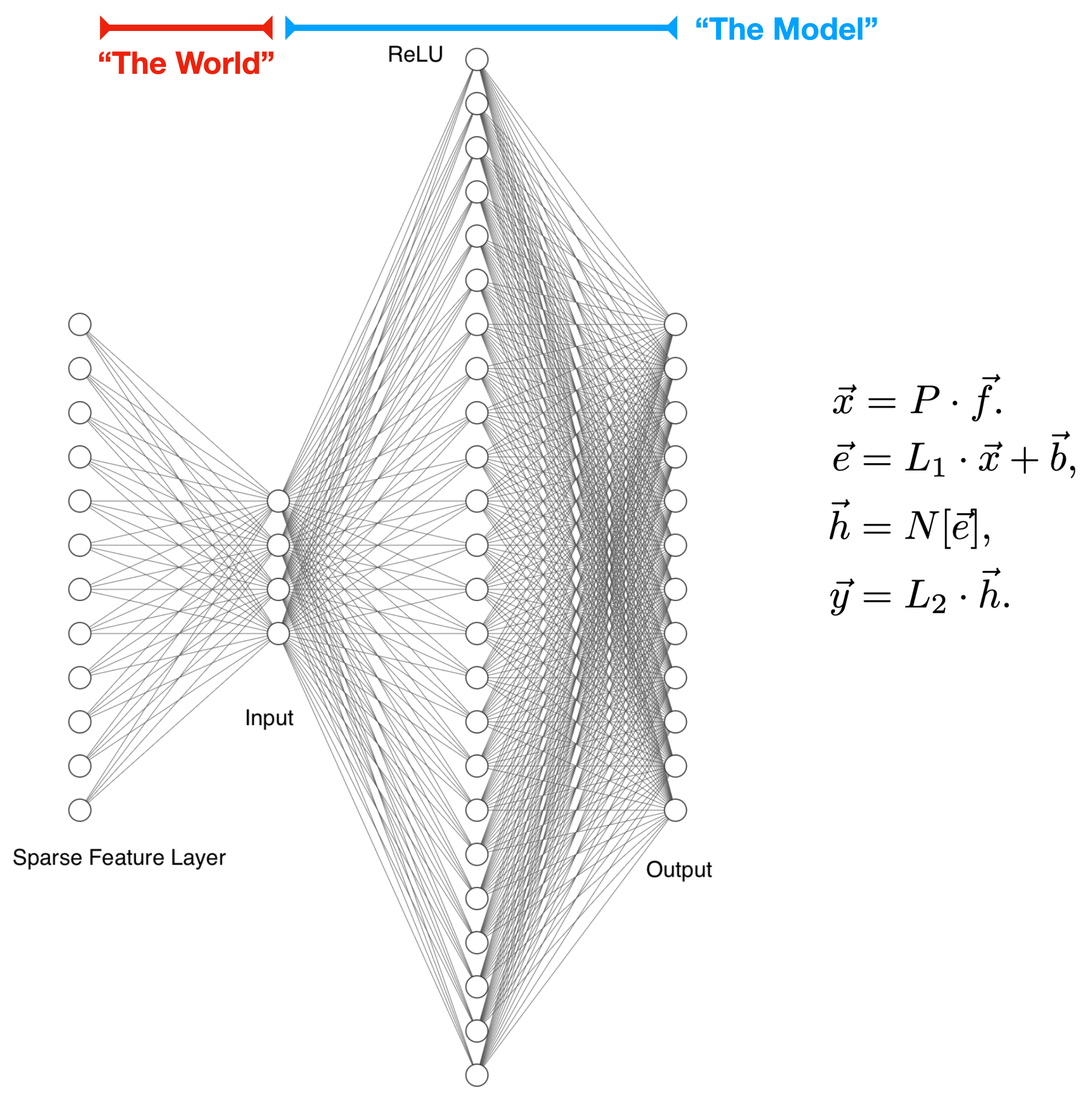
Features are generated as sparse vectors in a high-dimensional space. They are then run through a (fixed) random projection layer to produce the inputs into our model. We imagine this random projection process as an analogy to the way the world encodes features in our observations.

Within the model, the first layer is a linear transformation with a bias, followed by a nonlinearity. The second layer is a linear transformation with no bias.

Our toy model is most similar to that of Elhage+22, with a key difference being that the extra linear layer allows us to vary the number of neurons independent of the number of features or the input dimension.

We study this two model on three tasks. The first, a feature decoder, performs a compressed sensing reconstruction of features that were randomly and lossily projected into a low-dimensional space. The second, a random re-projector, reconstructs one fixed random projection of features from a different fixed random projection. The third, an absolute value calculator, performs the same compressed sensing task and then returns the absolute values of the recovered features. These tasks have the important property that we know which features are naturally useful, and so can easily measure the extent to which neurons are monosemantic or polysemantic.

Note that we primarily study the regime where there are more features than embedding dimensions (i.e. the sparse feature layer is wider than the input) but where features are sufficiently sparse that the number of features present in any given sample is smaller than the embedding dimension. We think this is likely the relevant limit for e.g. language models, where there are a vast array of possible features but few are present in any given sample.

Key Results

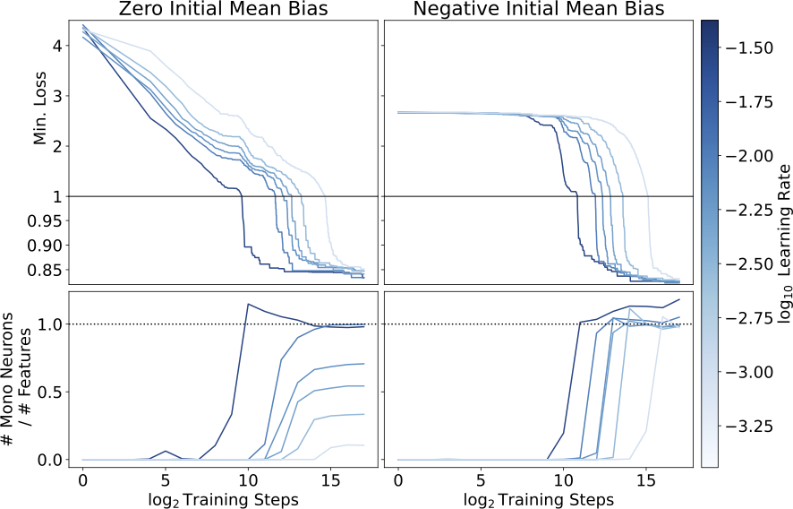
We find that models initialized with zero mean bias (left) find different local minima depending on the learning rate, with more monosemantic solutions and slightly lower loss at higher learning rates. Models initialized with a negative mean bias (right) all find highly monosemantic local minima, and achieve slightly better loss. Note that these models are all in a regime where they have more neurons than there are input features.

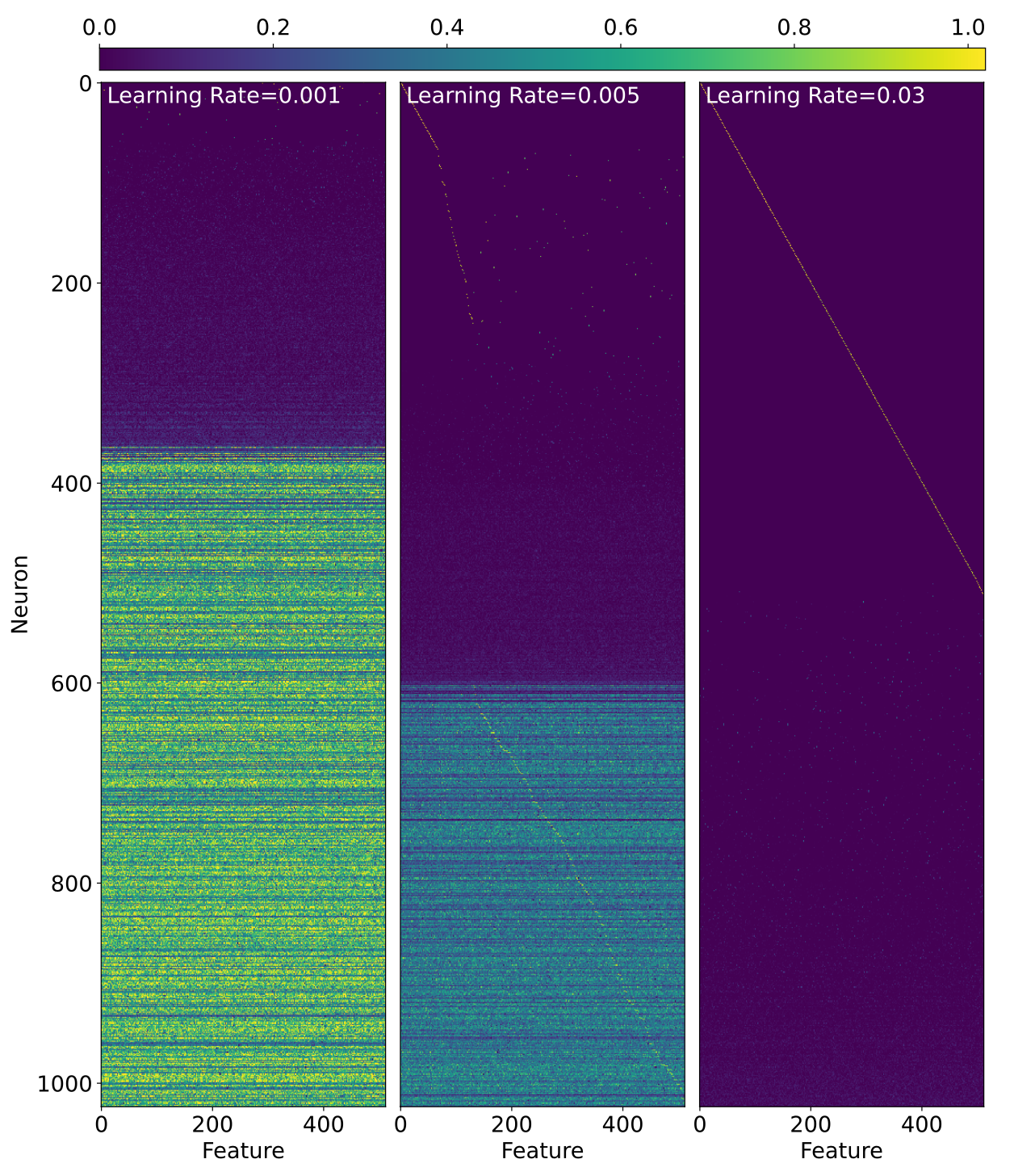
Just to hammer home how weird this is, below we've plotted the activations of neurons in response to single-feature inputs. The three models we show get essentially the same loss but are clearly doing very different things!

More generally, we find:

1. When inputs are feature-sparse, models can be made more monosemantic with no degredation in performance by just changing which loss minimum the training process finds (Section 4.1.1).
2. More monosemantic loss minima have moderate negative biases in all three tasks, and we are able to use this fact to engineer highly monosemantic models (Section 4.1.2).
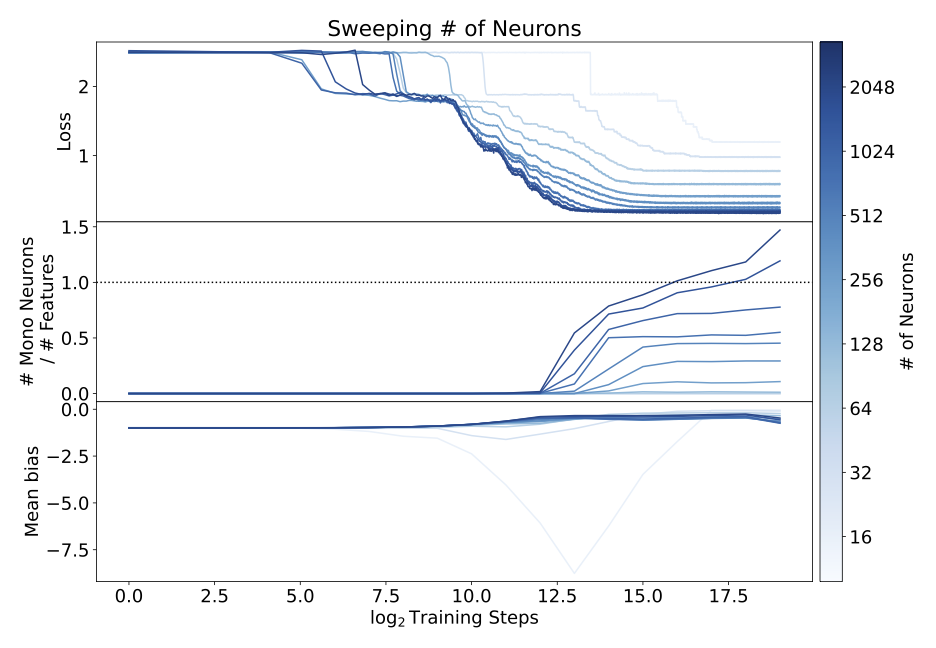
3. Providing models with more neurons per layer makes the models more monosemantic, albeit at increased computational cost (Section 4.1.4, also see below).

Interpretability

In Section 5 we provide some mechanistic interpretability results for our feature decoder models in the monosemantic limit. In this toy model setting we can decompose our model into a monosemantic part and a polysemantic part, and plotting these separately feature-by-feature is revealing:

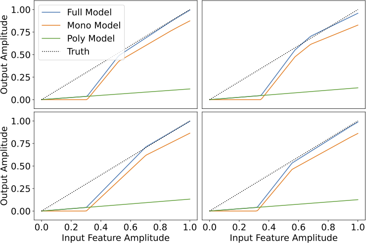
From this, we find that:

1. When there is a single monosemantic neuron for a feature, that neuron implements a simple algorithm of balancing feature recovery against interference.
2. When there are two monosemantic neurons for a feature, those neurons together implement an algorithm that classifies potential features as ``likely real'' or ``likely interference'', and then recovers the strength of any ``likely real'' features.

Additionally, we were suspicious at how few kinks the polysemantic neurons provided to the model's output. Indeed plotting the linearized map that these neurons implement reveals that they primarily serve to implement a low-rank approximation to the identity, which allows the model to have non-zero confidence in features at low input amplitudes: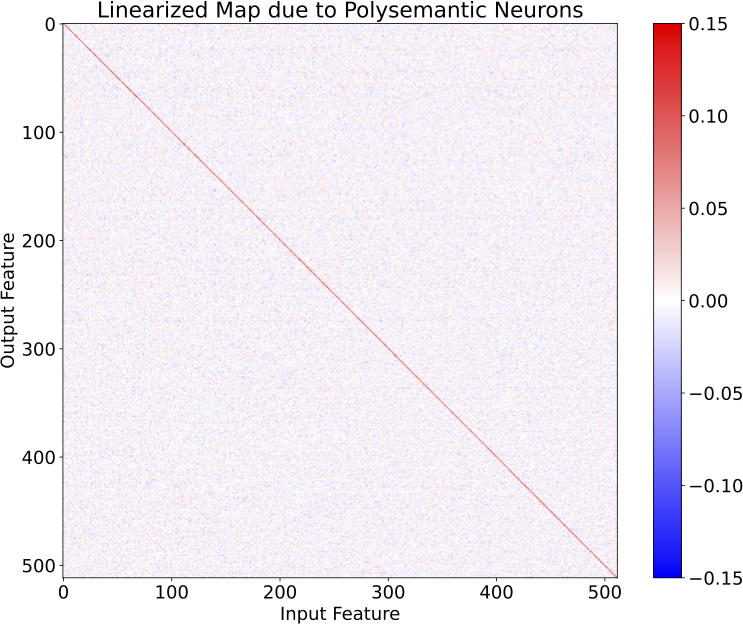

Future Work

We think there's a lot of low-hanging fruit in the direction of "engineer models to be more monosemantic", and we're excited to pick some more of it. The things we're most excited about include:

1. Our approach to engineering monosemanticity through bias could be made more robust by tailoring the bias weight decay on a per-neuron basis, or tying it to the rate of change of the rest of the model weights.
2. We've had some luck with an approach of the form "Engineer models to be more monosemantic, then interpret the remaining polysemantic neurons. Figure out what they do, re-architect the model to make that a monosemantic function, and interpret any new polysemantic neurons that emerge." We think we're building useful intuition playing this game, and are hopeful that there might be some more general lessons to be learned from it.
3. We have made naive attempts to use sparsity to reduce the cost of having more neurons per layer, but these degraded performance substantially. It is possible that further work in this direction will yield more workable solutions.

We'd be excited to answer questions about our work or engage with comments/suggestions for future work, so please don't be shy!

7 comments

Comments sorted by top scores.