Posts
Comments
As long as you make it clear at the header that it's your unofficial translation, go for it!
I would guess that models plan in this style much more generally. It's just useful in so many contexts. For instance, if you're trying to choose what article goes in front of a word, and that word is fixed by other constraints, you need a plan of what that word is ("an astronomer" not "a astronomer"). Or you might be writing code and have to know the type of the return value of a function before you've written the body of the function, since Python type annotations come at the start of the function in the signature. Etc. This sort of thing just comes up all over the place.
It's not so much that we didn't think models plan ahead in general, as that we had various hypotheses (including "unknown unknowns") and this kind of planning in poetry wasn't obviously the best one until we saw the evidence.
[More generally: in Interpretability we often have the experience of being surprised by the specific mechanism a model is using, even though with the benefit of hindsight it seems obvious. E.g. when we did the work for Towards Monosemanticity we were initially quite surprised to see the "the in <context>" features, thought they were indicative of a bug in our setup, and had to spend a while thinking about them and poking around before we realized why the model wanted them (which now feels obvious).]
I can also confirm (I have a 3:1 match).
Unless we build more land (either in the ocean or in space)?
There is Dario's written testimony before Congress, which mentions existential risk as a serious possibility: https://www.judiciary.senate.gov/imo/media/doc/2023-07-26_-_testimony_-_amodei.pdf
He also signed the CAIS statement on x-risk: https://www.safe.ai/work/statement-on-ai-risk
He does start out by saying he thinks & worries a lot about the risks (first paragraph):
I think and talk a lot about the risks of powerful AI. The company I’m the CEO of, Anthropic, does a lot of research on how to reduce these risks... I think that most people are underestimating just how radical the upside of AI could be, just as I think most people are underestimating how bad the risks could be.
He then explains (second paragraph) that the essay is meant to sketch out what things could look like if things go well:
In this essay I try to sketch out what that upside might look like—what a world with powerful AI might look like if everything goes right.
I think this is a coherent thing to do?
I get 1e7 using 16 bit-flips per bfloat16 operation, 300K operating temperature, and 312Tflop/s (from Nvidia's spec sheet). My guess is that this is a little high because a float multiplication involves more operations than just flipping 16 bits, but it's the right order-of-magnitude.
Another objection is that you can minimize the wrong cost function. Making "cost" go to zero could mean making "the thing we actually care about" go to (negative huge number).
One day a mathematician doesn’t know a thing. The next day they do. In between they made no observations with their senses of the world.
It’s possible to make progress through theoretical reasoning. It’s not my preferred approach to the problem (I work on a heavily empirical team at a heavily empirical lab) but it’s not an invalid approach.
I'm guessing that the sales numbers aren't high enough to make $200k if sold at plausible markups?
In Towards Monosemanticity we also did a version of this experiment, and found that the SAE was much less interpretable when the transformer weights were randomized (https://transformer-circuits.pub/2023/monosemantic-features/index.html#appendix-automated-randomized).
Anthropic’s RSP includes evals after every 4x increase in effective compute and after every 3 months, whichever comes sooner, even if this happens during training, and the policy says that these evaluations include fine-tuning.
This matches my impression. At EAG London I was really stunned (and heartened!) at how many skilled people are pivoting into interpretability from non-alignment fields.
Second, the measure of “features per dimension” used by Elhage et al. (2022) might be misleading. See the paper for details of how they arrived at this quantity. But as shown in the figure above, “features per dimension” is defined as the Frobenius norm of the weight matrix before the layer divided by the number of neurons in the layer. But there is a simple sanity check that this doesn’t pass. In the case of a ReLU network without bias terms, multiplying a weight matrix by a constant factor will cause the “features per dimension” to be increased by that factor squared while leaving the activations in the forward pass unchanged up to linearity until a non-ReLU operation (like a softmax) is performed. And since each component of a softmax’s output is strictly increasing in that component of the input, scaling weight matrices will not affect the classification.
It's worth noting that Elhage+2022 studied an autoencoder with tied weights and no softmax, so there isn't actually freedom to rescale the weight matrix without affecting the loss in their model, making the scale of the weights meaningful. I agree that this measure doesn't generalize to other models/tasks though.
They also define a more fine-grained measure (the dimensionality of each individual feature) in a way that is scale-invariant and which broadly agrees with their coarser measure...
I think there’s tons of low-hanging fruit in toy model interpretability, and I expect at least some lessons from at least some such projects to generalize. A lot of the questions I’m excited about in interpretability are fundamentally accessible in toy models, like “how do models trade off interference and representational capacity?”, “what priors do MLP’s have over different hypotheses about the data distribution?”, etc.
A thing I really like about the approach in this paper is that it makes use of a lot more of the model's knowledge of human values than traditional RLHF approaches. Pretrained LLM's already know a ton of what humans say about human values, and this seems like a much more direct way to point models at that knowledge than binary feedback on samples.
How does this correctness check work?
I usually think of gauge freedom as saying “there is a family of configurations that all produce the same observables”. I don’t think that gives a way to say some configurations are correct/incorrect. Rather some pairs of configurations are equivalent and some aren’t.
That said, I do think you can probably do something like the approach described to assign a label to each equivalence class of configurations and do your evolution in that label space, which avoids having to pick a gauge.
How would you classify optimization shaped like "write a program to solve the problem for you". It's not directly searching over solutions (though the program you write might). Maybe it's a form of amortized optimization?
Separately: The optimization-type distinction clarifies a circle I've run around talking about inner optimization with many people, namely "Is optimization the same as search, or is search just one way to get optimization?" And I think this distinction gives me something to point to in saying "search is one way to get (direct) optimization, but there are other kinds of optimization".
I might be totally wrong here, but could this approach be used to train models that are more likely to be myopic (than e.g. existing RL reward functions)? I'm thinking specifically of the form of myopia that says "only care about the current epoch", which you could train for by (1) indexing epochs, (2) giving the model access to its epoch index, (3) having the reward function go negative past a certain epoch, (4) giving the model the ability to shutdown. Then you could maybe make a model that only wants to run for a few epochs and then shuts off, and maybe that helps avoid cross-epoch optimization?
That's definitely a thing that can happen.
I think the surgeon can always be made ~arbitrarily powerful, and the trick is making it not too powerful/trivially powerful (in ways that e.g. preclude the model from performing well despite the surgeon's interference).
So I think the core question is: are there ways to make a sufficiently powerful surgeon which is also still defeasible by a model that does what we want?
A trick I sometimes use, related to this post, is to ask whether my future self would like to buy back my present time at some rate. This somehow makes your point about intertemporal substitution more visceral for me, and makes it easier to say "oh yes this thing which is pricier than my current rate definitely makes sense at my plausible future rate".
In fact, it's not 100% clear that AI systems could learn to deceive and manipulate supervisors even if we deliberately tried to train them to do it. This makes it hard to even get started on things like discouraging and detecting deceptive behavior.
Plausibly we already have examples of (very weak) manipulation, in the form of models trained with RLHF saying false-but-plausible-sounding things, or lying and saying they don't know something (but happily providing that information in different contexts). [E.g. ChatGPT denies having information about how to build nukes, but will also happily tell you about different methods for Uranium isotope separation.]
Yeah. Or maybe not even to zero but it isn’t increasing.
Could it be that Chris's diagram gets recovered if the vertical scale is "total interpretable capabilities"? Like maybe tiny transformers are more interpretable in that we can understand ~all of what they're doing, but they're not doing much, so maybe it's still the case that the amount of capability we can understand has a valley and then a peak at higher capability.
That's a good point: it definitely pushes in the direction of making the model's internals harder to adversarially attack. I do wonder how accessible "encrypted" is here versus just "actually robust" (which is what I'm hoping for in this approach). The intuition here is that you want your model to be able to identify that a rogue thought like "kill people" is not a thing to act on, and that looks like being robust.
And: having a lot of capital could be very useful in the run up to TAI. Eg for pursuing/funding safety work.
Roughly, I think it’s hard to construct a reward signal that makes models answer questions when they know the answers and say they don’t know when they don’t know. Doing that requires that you are always able to tell what the correct answer is during training, and that’s expensive to do. (Though Eg Anthropic seems to have made some progress here: https://arxiv.org/abs/2207.05221).
So indeed with cross-entropy loss I see two plateaus! Here's rank 2:
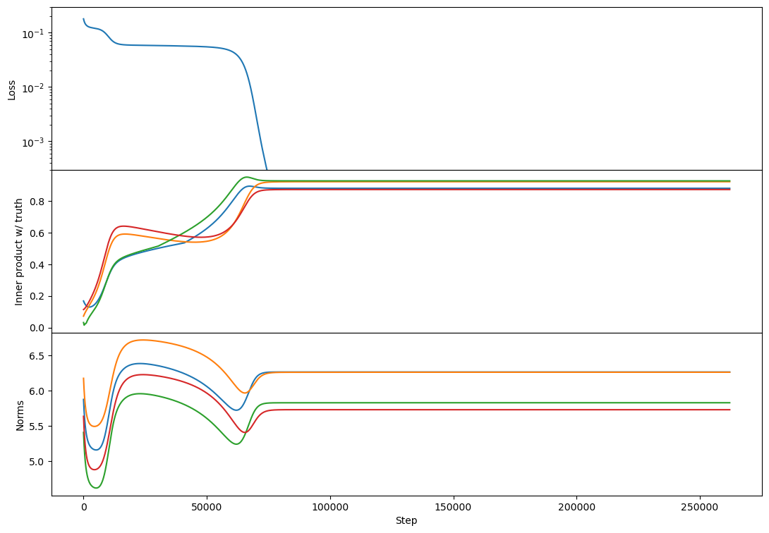
(note that I've offset the loss to so that equality of Z and C is zero loss)
I have trouble getting rank 10 to find the zero-loss solution:
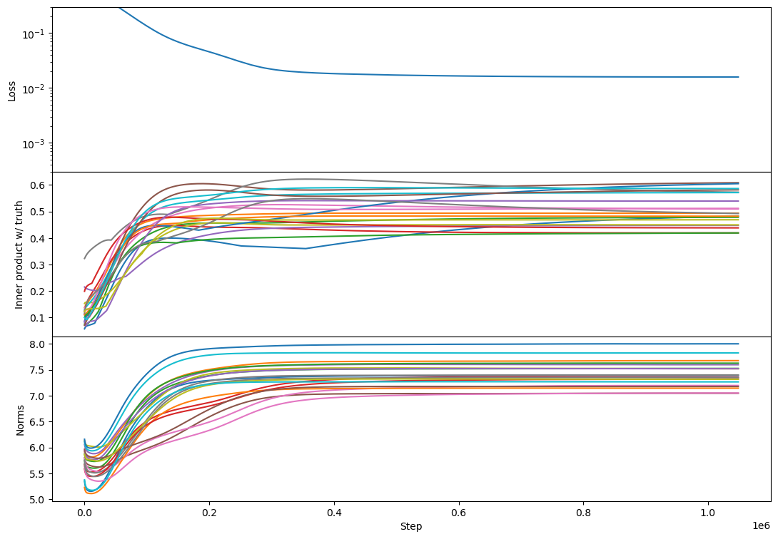
But the phenomenology at full rank is unchanged:
Got it, I see. I think of the two as really intertwined (e.g. a big part of my agenda at the moment is studying how biases/path-dependence in SGD affect interpretability/polysemanticity).
This is really interesting!
One question: do we need layer norm in networks? Can we get by with something simpler? My immediate reaction here is “holy cow layer norm is geometrically complicated!” followed by a desire to not use it in networks I’m hoping to interpret.
This post introduces the concept of a "cheerful price" and (through examples and counterexamples) narrows it down to a precise notion that's useful for negotiating payment. Concretely:
- Having "cheerful price" in your conceptual toolkit means you know you can look for the number at which you are cheerful (as opposed to "the lowest number I can get by on", "the highest number I think they'll go for", or other common strategies). If you genuinely want to ask for an amount that makes you cheerful and no more, knowing that such a number might exist at all is useful.
- Even if you might want to ask for more than your cheerful price, your cheerful price helps bound how low you want the negotiation to go (subject to constraints listed in the post, like "You need to have Slack").
- If both parties know what "cheerful price" means it's way easier to have a negotiation that leaves everyone feeling good by explicitly signaling "I will feel less good if made to go below this number, but amounts above this number don't matter so much to me." That's not the way to maximize what you get, but that's often not the goal in a negotiation and there are other considerations (e.g. how people feel about the transaction, willingness to play iterated games, etc.) that a cheerful price does help further.
The other cool thing about this post is how well human considerations are woven in (e.g. inner multiplicity, the need for safety margins, etc.). The cheerful price feels like a surprisingly simple widget given how much it bends around human complexity.
I found this post a delightful object-level exploration of a really weird phenomenon (the sporadic occurrence of the "tree" phenotype among plants). The most striking line for me was:
Most “fruits” or “berries” are not descended from a common “fruit” or “berry” ancestor. Citrus fruits are all derived from a common fruit, and so are apples and pears, and plums and apricots – but an apple and an orange, or a fig and a peach, do not share a fruit ancestor.
What is even going on here?!
On a meta-level my takeaway was to be a bit more humble in saying what complex/evolved/learned systems should/shouldn't be capable of/do.
Woah, nice! Note that I didn't check rank 1 with Adam, just rank >= 2.
Erm do C and Z have to be valid normalized probabilities for this to work?
Got it, I was mostly responding to the third paragraph (insight into why SGD works, which I think is mostly an interpretability question) and should have made that clearer.
(with the caveat that this is still "I tried a few times" and not any quantitative study)
It's a good caution, but I do see more bumps with Adam than with SGD across a number of random initializations.
Something like this?
def loss(learned, target):
p_target = torch.exp(target)
p_target = p_target / torch.sum(p_target)
p_learned = torch.exp(learned)
p_learned = p_learned / torch.sum(p_learned)
return -torch.sum(p_target * torch.log(p_learned))
I'd be very excited to see a reproduction :-)
This problem is not neglected, and it is very unclear how any insight into why SGD works wouldn’t be directly a capabilities contribution.
I strongly disagree! AFAICT SGD works so well for capabilities that interpretability/actually understanding models/etc. is highly neglected and there's low-hanging fruit all over the place.
I don't think so? I think that just means you keep the incorrect initialization around while also learning the correct direction.
I agree with both of your rephrasings and I think both add useful intuition!
Regarding rank 2, I don't see any difference in behavior from rank 1 other than the "bump" in alignment that Lawrence mentioned. Here's an example:
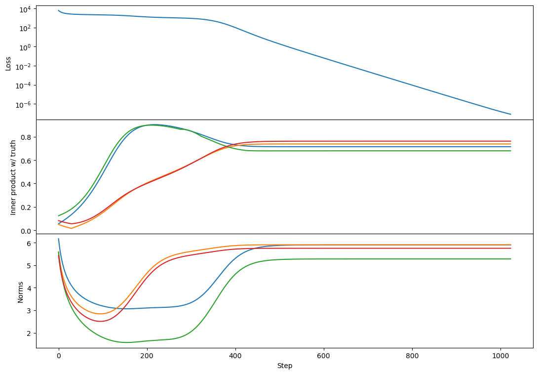
This doesn't happen in all rank-2 cases but is relatively common. I think usually each vector grows primarily towards 1 or the other target. If two vectors grow towards the same target then you get this bump where one of them has to back off and align more towards a different target [at least that's my current understanding, see my reply to Lawrence for more detail!].
What happens in a cross-entropy loss style setup, rather than MSE loss? IMO cross-entropy loss is a better analogue to real networks. Though I'm confused about the right way to model an internal sub-circuit of the model. I think the exponential decay term just isn't there?
What does a cross-entropy setup look like here? I'm just not sure how to map this toy model onto that loss (or vice-versa).
How does this interact with weight decay? This seems to give an intrinsic exponential decay to everything
Agreed! I expect weight decay to (1) make the converged solution not actually minimize the original loss (because the weight decay keeps tugging it towards lower norms) and (2) accelerate the initial decay. I don't think I expect any other changes.
How does this interact with softmax? Intuitively, softmax feels "S-curve-ey"
I'm not sure! Do you have a setup in mind?
How does this with interact with Adam? In particular, Adam gets super messy because you can't just disentangle things. Even worse, how does it interact with AdamW?
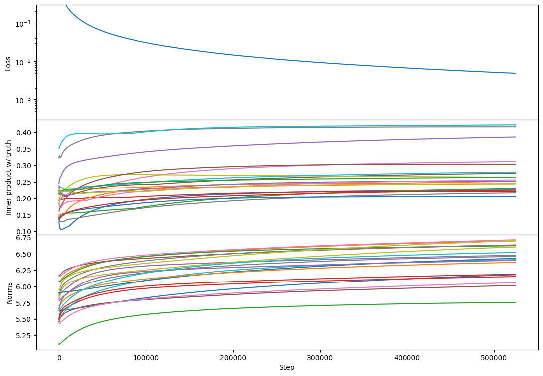
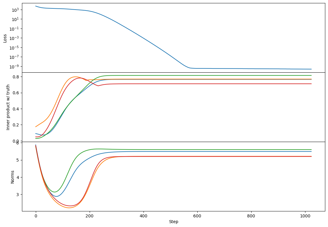
I agree this breaks my theoretical intuition. Experimentally most of the phenomenology is the same, except that the full-rank (rank 100) case regains a plateau.
Here's rank 2:
rank 10:
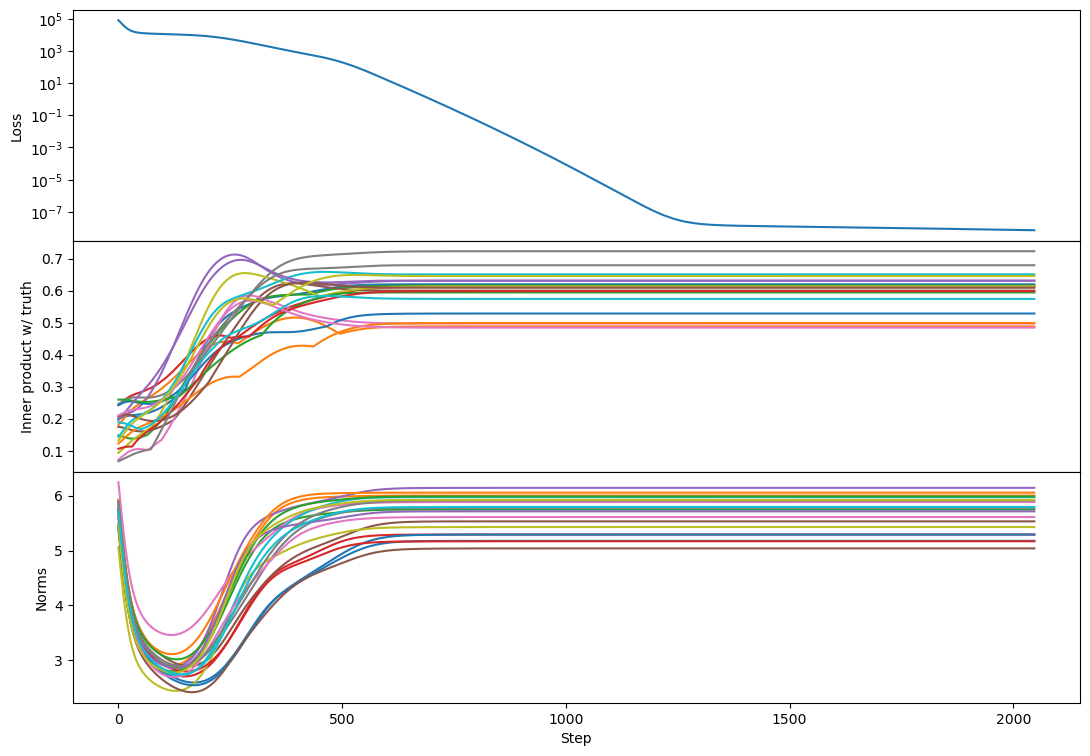
(maybe there's more 'bump' formation here than with SGD?)
rank 100:
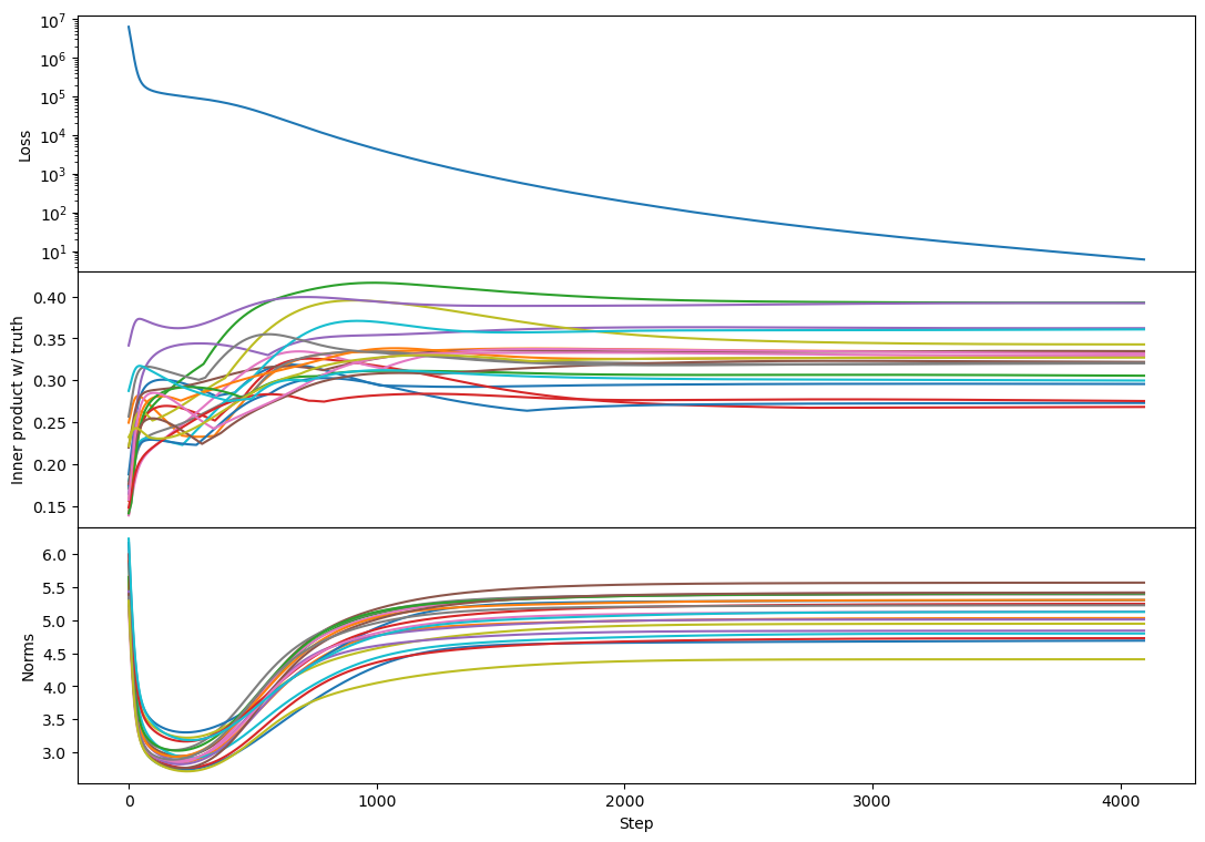
It kind of looks like the plateau has returned! And this replicates across every rank 100 example I tried, e.g.
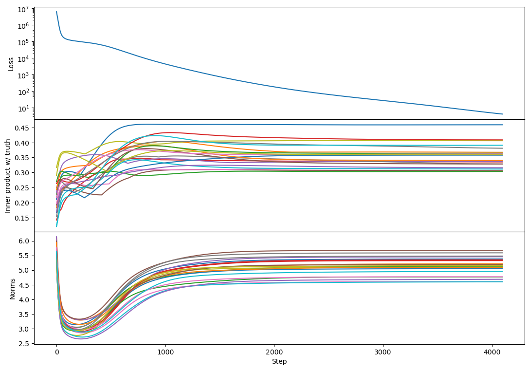
The plateau corresponds to a period with a lot of bump formation. If bumps really are a sign of vectors competing to represent different chunks of subspace then maybe this says that Adam produces more such competition (maybe by making different vectors learn at more similar rates?).
I'd be curious if you have any intuition about this!
I don't, but here's my best guess: there's a sense in which there's competition among vectors for which learned vectors capture which parts of the target span.
As a toy example, suppose there are two vectors, and , such that the closest target vector to each of these at initialization is . Then both vectors might grow towards . At some point is represented enough in the span, and it's not optimal for two vectors to both play the role of representing , so it becomes optimal for at least one of them to shift to cover other target vectors more.
For example, from a rank-4 case with a bump, here's the inner product with a single target vector of two learned vectors:
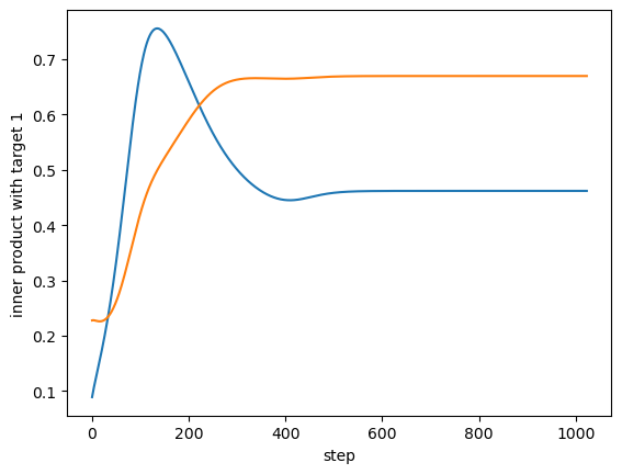
So both vectors grow towards a single target, and the blue one starts realigning towards a different target as the orange one catches up.
Two more weak pieces of evidence in favor of this story:
- We only ever see this bump when the rank is greater than 1.
- From visual inspection, bumps are more likely to peak at higher levels of alignment than lower levels, and don't happen at all in initial norm-decay phase, suggesting the bump is associated with vectors growing (rather than decaying).
This is really interesting! One extension that comes to mind: SVD will never recover a Johnson-Lindenstrauss packing, because SVD can only return as many vectors as the rank of the relevant matrix. But you can do sparse coding to e.g. construct an overcomplete basis of vectors such that typical samples are sparse combinations of those vectors. Have you tried/considered trying something like that?
That's not a scalar, do you mean the trace of that? If so, doesn't that just eliminate the term that causes the incorrect initialization to decay?
Good catch, fixed!
Ah that's right. Will edit to fix.
Do you have results with noisy inputs?
Nope! Do you have predictions for what noise might do here?
The negative bias lines up well with previous sparse coding implementations: https://scholar.google.com/citations?view_op=view_citation&hl=en&user=JHuo2D0AAAAJ&citation_for_view=JHuo2D0AAAAJ:u-x6o8ySG0sC
Oooo I'll definitely take a look. This looks very relevant.
Note that in that research, the negative bias has a couple of meanings/implications:
- It should correspond to the noise level in your input channel.
- Higher negative biases directly contribute to the sparsity/monosemanticty of the network.
We don't have any noise, but we do think that the bias is serving a de-interference role (because features get packed together in a space that's not big enough to avoid interference).
Along those lines, you might be able to further improve monosemanticity by using the lasso loss function.
Can you say more about why? We know that L1 regularization on the activations (or weights) increases monosemanticity, but why do you think this would happen when done as part of the task loss?
Thanks for these thoughts!
Although it would be useful to have the plotting code as well, if that's easy to share?
Sure! I've just pushed the plot helper routines we used, as well as some examples.
I agree that N (true feature dimension) > d (observed dimension), and that sparsity will be high, but I'm uncertain whether the other part of the regime (that you don't mention here), that k (model latent dimension) > N, is likely to be true. Do you think that is likely to be the case? As an analogy, I think the intermediate feature dimensions in MLP layers in transformers (analogously k) are much lower dimension than the "true intrinsic dimension of features in natural language" (analogously N), even if it is larger than the input dimension (embedding dimension* num_tokens, analogously d). So I expect
This is a great question. I think my expectation is that the number of features exceeds the number of neurons in real-world settings, but that it might be possible to arrange for the number of neurons to exceed the number of important features (at least if we use some sparsity/gating methods to get many more neurons without many more flops).
If we can't get into that limit, though, it does seem important to know what happens when k < N, and we looked briefly at that limit in section 4.1.4. There we found that models tend to learn some features monosemantically and others polysemantically (rather than e.g. ignoring all but k features and learning those monosemantically), both for uniform and varying feature frequencies.
This is definitely something we want to look into more though, in particular in case of power-law (or otherwise varying) feature frequencies/importances. You might well expect that features just get ignored below some threshold and monosemantically represented above it, or it could be that you just always get a polysemantic morass in that limit. We haven't really pinned this down, and it may also depend on the initialization/training procedure (as we saw when k > N), so it's definitely worth a thorough look.
In the paper you say that you weakly believe that monosemantic and polysemantic network parametrisations are likely in different loss basins, given they're implementing very different algorithms. I think (given the size of your networks) it should be easy to test for at least linear mode connectivity with something like git re-basin (https://github.com/samuela/git-re-basin).
We haven't tried this. It's something we looked into briefly but were a little concerned about going down a rabbit hole given some of the discussion around whether the results replicated, which indicated some sensitivity to optimizer and learning rate.
I think (at least in our case) it might be simpler to get at this question, and I think the first thing I'd do to understand connectivity is ask "how much regularization do I need to move from one basin to the other?" So for instance suppose we regularized the weights to directly push them from one basin towards the other, how much regularization do we need to make the models actually hop?
Actually, one related reason we think that these basins are unlikely to be closely connected is that we see the monosemanticity "converge" towards the end of long training runs, rather than e.g. drifting as the model moves along a ridge. We don't see this convergence everywhere, and in particular in high-k power-law models we see continuing evolution after many steps, but we think we understand that as a refinement of a particular minimum to better capture infrequent features.
You also mentioned your initial attempts at sparsity through a hard-coded initially sparse matrix failed; I'd be very curious to see whether a lottery ticket-style iterative magnitude pruning was able to produce sparse matrices from the high-latent-dimension monosemantic networks that are still monosemantic, or more broadly how the LTH interacts with polysemanticity - are lottery tickets less polysemantic, or more, or do they not really change the monosemanticity?
Good question! We haven't tried that precise experiment, but have tried something quite similar. Specifically, we've got some preliminary results from a prune-and-grow strategy (holding sparsity fixed, pruning smallest-magnitude weights, enabling non-sparse weights) that does much better than a fixed sparsity strategy.
I'm not quite sure how to interpret these results in terms of the lottery ticket hypothesis though. What evidence would you find useful to test it?