Input Swap Graphs: Discovering the role of neural network components at scale
post by Alexandre Variengien (alexandre-variengien) · 2023-05-12T09:41:08.800Z · LW · GW · 0 commentsContents
  A five-minute overview of swap graphs
    Motivation
    A short high-level description
    A toy example
    Practical implementation
    Experimental Results on a Name Mover Head
    Takeaways
  A theoretical setting: reverse-engineering from causal interventions
    Problem setting
    The naive interpretation of swap graphs
    Counterexamples to the naive interpretation of swap graphs
        Swap graphs can contain strictly directed edges.
        Swap graphs can contain strictly directed edges even when filtering for dependency.
        Cliques in swap graphs don’t map to variable values in the program.
    Takeaways to interpret swap graphs in practice
      Takeaways from the counterexamples
      A (hand-wavy) frequency argument to design datasets that favor the naive interpretation
      The empirical naive interpretation
    Extension of the theoretical setting
  Comparative LM anatomy: studying the IOI task in multibillion parameter models
    Manual study of IOI on GPT2-small
      Technical implementation
      Swap graphs deeper into the IOI circuit
        Name Mover's queries.
        S-Inhibition heads.
        Going deeper: duplicate token heads and induction heads.
      Surprising results in a Mistral model and GPT2-small: gendered S-Inhibition heads.
    Scaling to larger models
        Observations/comments
        Semantic maps of queries.
    Validation of swap graphs in larger models
      Causal Scrubbing: resampling inside the communities
        Scrubbing baselines.
        Comparing partitions
        Experiment results.
        Observations/comments
      Targeted rewriting: patching across communities
        Targetted rewrite on Name Movers
        Targetted rewrites of senders components
        Observations/comments:
  Limitations and future work
    Takeaways
        Swap graphs for exploratory interp
        Toy theoretical model of localized computation
        Swap graphs to understand large models
    Future works
  Appendix: Swap graph with logit difference
None
No comments
This post was written as part of the work done at Conjecture.
You can try input swap graphs in a collab notebook or explore the library to replicate the results.
Thanks to Beren Millidge and Eric Winsor for useful discussions throughout this project. Thanks to Beren for feedback on a draft of this post.
Activation and path patching are techniques employed to manipulate neural network internals. One approach, used in ROME, which we'll refer to as corrupted patching, involves setting the output of certain parts of the network to a corrupted value. Another method used in the work on indirect object identification, referred to as input swap patching, involves assigning these parts the values they would produce on a different input sample, while the rest of the model operates normally. These experimental techniques have proven effective in gaining structural insights into the information flow within neural networks, providing a better understanding of which components are involved in a given behavior. These structural analyses can be straightforwardly automated using algorithms like Automatic Circuit DisCovery.
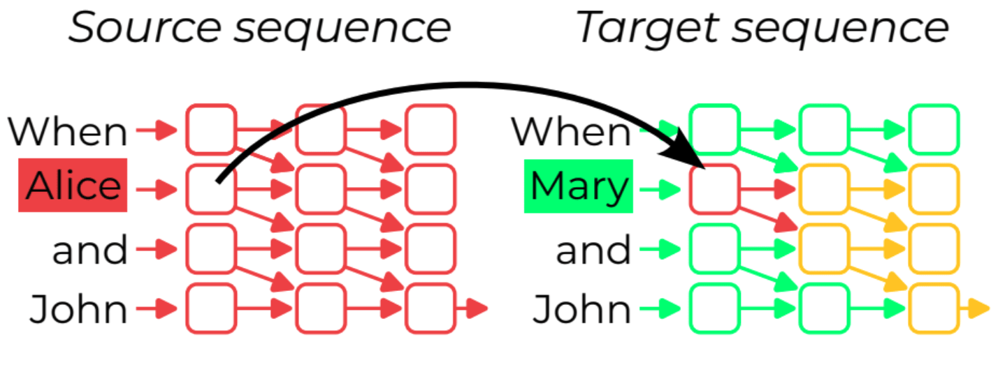
Patching experiments also enable the discovery of the semantics of components, i.e. the abstract variables a component encodes. They have been used to discover the "a vs an" neuron in gpt2 [LW · GW], the token and position signal in S-inhibition heads in the IOI circuit, or Othello board representations [LW · GW]. In all these cases, researchers were not only able to say 'this component matters', but also 'it roughly plays this role'. However, these additional results come at a cost: they often required a lot of manual effort to design alternative datasets and come up with an intuition for the likely role of the component in advance.
In this post, I introduce input swap graphs (swap graphs in short), a new tool to systematically analyze the results of input swap patching experiments and recover semantic information with as little human effort as possible.
In the following, I present
- A concise overview of swap graphs, their motivation, and practical application to Name Movers within the IOI circuit.
- A simple theoretical framework for examining the problem of localized computation in computational graphs. This framework serves as a sandbox for rapidly building intuition to create or interpret experiments, such as swap graphs, which can be applied to real-world neural networks.
- An expansion of the IOI study in GPT-2 small to models containing several billion parameters (GPT-2 XL, Pythia-2.8B, GPT-Neo-2.7B) using swap graphs. We validated our findings through causal scrubbing [LW · GW] and targeted interventions that steer the mechanism out-of-distribution predictably. This both demonstrates the potential for applying swap graphs to larger models and presents valuable data to investigate how a model's internal structure changes with scale while performing the same task.
A five-minute overview of swap graphs
Motivation
Deciphering the intermediate activations of neural network components can be a daunting task. The prevalent approach involves breaking down these high-dimensional vectors into subspaces where variations correspond to concepts that are both relevant to the model's computation and comprehensible to humans.
In this work, we adopt an alternative strategy: we limit ourselves to using only input swap patching in order to uncover the roles of neural network components without directly exploiting the structure of their activations.
While it is common to combine information about directions in activation space and input swap patching experiments in interpretability research (e.g., as demonstrated in Neel Nanda's work on Othello [LW · GW]), our objective here is to investigate the extent to which we can rely solely on input swap patching. This motivation is twofold: i) gaining a clearer understanding of the insights offered by different techniques, and ii) capitalizing on the simplicity of input swap patching, which can be readily translated into causal scrubbing experiments and modifications of the model's behavior. By maximizing our discoveries using patching alone, we remain closer to the experiments that matter most and reduce the risk of misleading ourselves along the way.
A short high-level description
Our aim is to create a comprehensible abstraction of the roles played by a model's subcomponents. For a given model component and a dataset, we ask: what role is it playing in the model computation? What abstract variables is it encoding?
We address this question by conducting input swap patching where we swap the input to , while maintaining the input to the rest of the model.
If swapping the input to does not change the model's output (verified by checking the small distance between the outputs before and after the swap), it may sometimes be because the component's output is interpreted in the same way by the subsequent model layers.
We do not have completely characterize the conditions under which we can naively interpret "no change in output" as "the component encodes the same value" rather than, for example, "the component's encoded value changed but the model output remained the same by coincidence". However, the naive interpretation seems empirically and theoretically reliable when the component can only encode a limited number of discrete values.
By running all possible input swaps (i.e., every pair of inputs ) and measuring the change in the model's output for each, we can organize the results into an input swap graph (shorten in swap graph hereafter). This graph has nodes representing dataset elements and edges that store the outcome of swapping for as input to .
We can identify communities in this graph, i.e., inputs that can be swapped with one another as input to without affecting the model's output. We then look for input features that remain constant within each community but vary between them. These findings significantly limit the possible abstract variables that can encode, as any candidate variable should respond to the input features in the same manner.
Consequently, swap graphs enable us to rapidly formulate hypotheses that can be further validated through more rigorous experiments like causal scrubbing [AF · GW] or refined by adjusting the dataset.
A toy example
Let’s take the example of a model being a processor implementing a simple function.
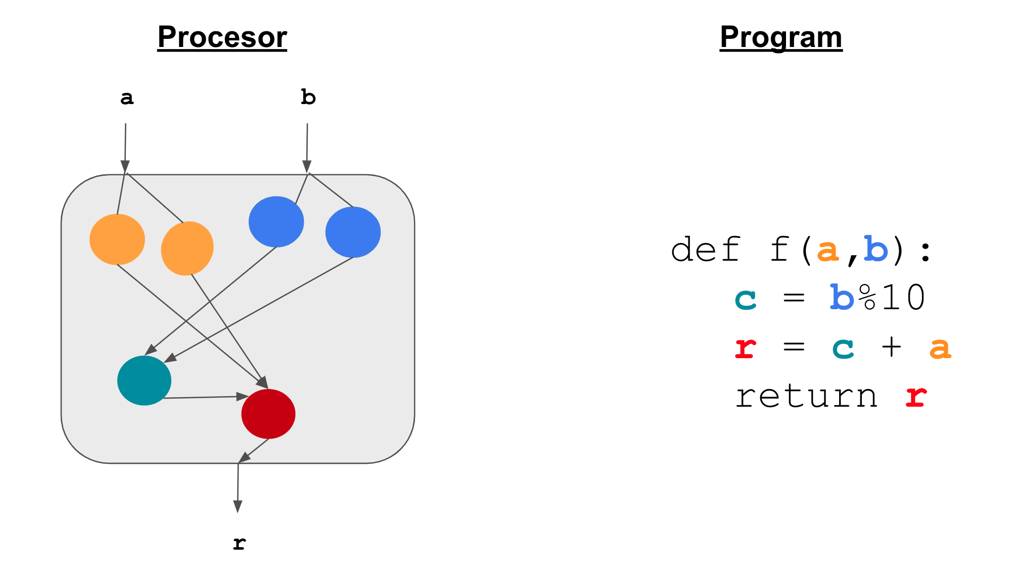
We’ll focus on understanding the role of the teal component. In the figure below, we swapped its input from (a=12, b=30) to (a=23, b=11).
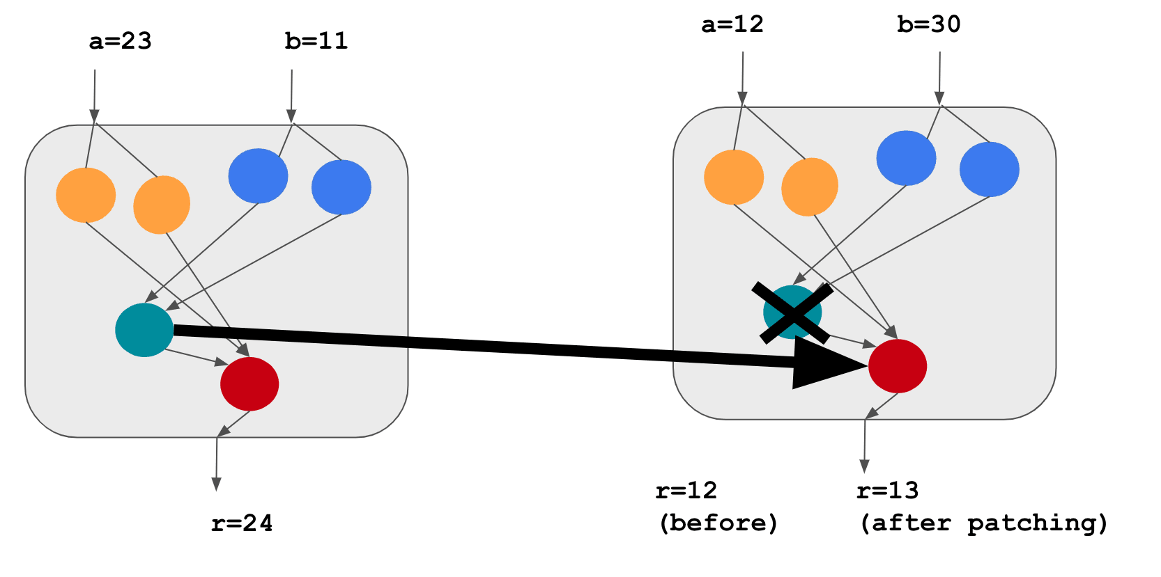
As the teal component encodes the program variable c, and that c=1 on the left run but 0 on the right run, patching the teal component makes the results on the right go from 12 to 13.
One single patching experiment is not very informative to obtain a comprehensive view of the role of a component, we need more of them!
Here is what the swap graph of the teal component looks like on a dataset of 7 inputs. We show the edges where the swap did not change the output of the model.
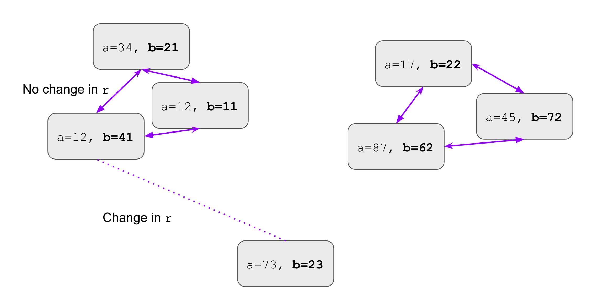
By observing the connected components of the graph, we can eyeball at what the inputs have in common: the fact that b%10 is the same in each of them! Hence, a reasonable guess is that the teal component encodes the intermediate variable b%10. We were able to find its role without access to the program.
Practical implementation
def swap_graph(
	D, # The dataset
	Comp, # The comparison function
	M, # The model
	C # The component to investigate
):
	"""Returns the swap graph of C on D."""
	G = np.empty(|D|, |D|) # The weight matrix of the swap graph
	for x,y in D:
 		G[x,y] = Comp(M(x), M(C(y), x)) # Measure how much the model output
 										# changes by swapping x by y as input to C
	return G
In practice, throughout this work, we used the KL divergence between the next-token probability distributions outputted by the original and the patched model as the Comp function. We transformed the distances given by the KL divergence into similarities using a Gaussian kernel.
The algorithm requires a quadratic number of forward passes in the number of dataset examples. It is tractable for a dataset size of around a hundred samples. Such sizes are enough to recover interesting structures on simple datasets such as IOI.
Once we have G, we can leverage classic network analysis such as:
- Force-directed visualization for manual inspection. We can eyeball the fit between the position found by force-directed layouts and hypothesized input feature. These visualizations can expose outliers, i.e. inputs where the component is probably doing something different from the rest of the dataset.
- Unsupervised community detection. We can automatize the previous step using algorithms such as the Louvain Method. Once we compute the communities, we can measure correlation with hypothesized abstract values the component could be encoding.
However, it's still unclear what information exactly we can recover from swap graphs (see next section below), and how to interpret them in the general case. When applied to IOI, we found that a naive interpretation was enough to recover results that were found with alternative methods.
Experimental Results on a Name Mover Head
Here is the IOI circuit found in GPT2-small: (for context on the IOI task and terminology, you can read the IOI paper or the last slides of this slideshow)
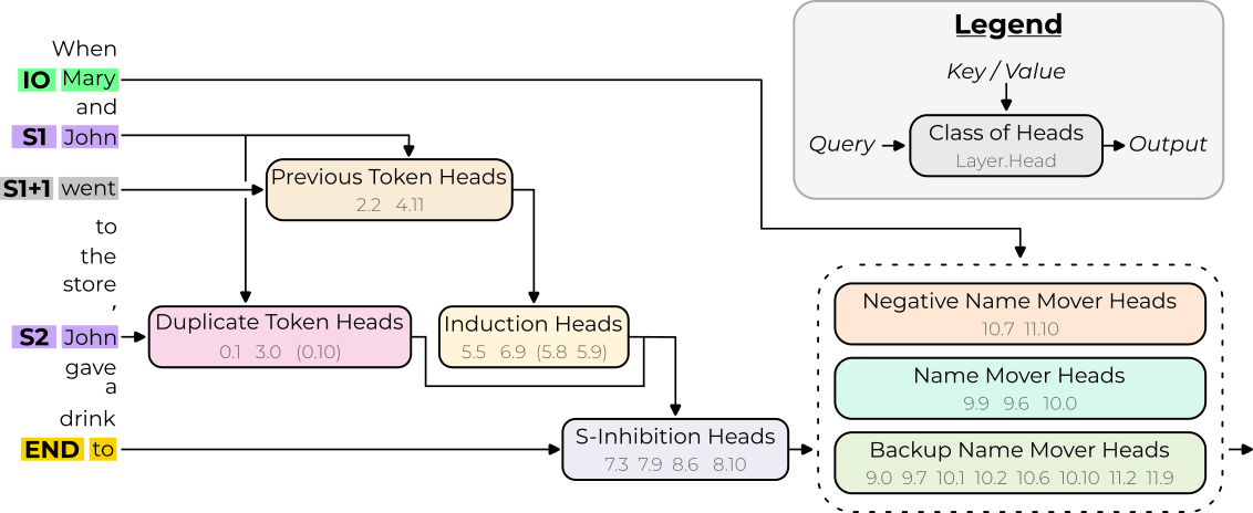
In the IOI paper, we characterize Name Movers as a class of heads acting as the “return” statement of the circuit.
Let’s compute the swap graph of the head 9.9 and visualize it with a force-directed layout.
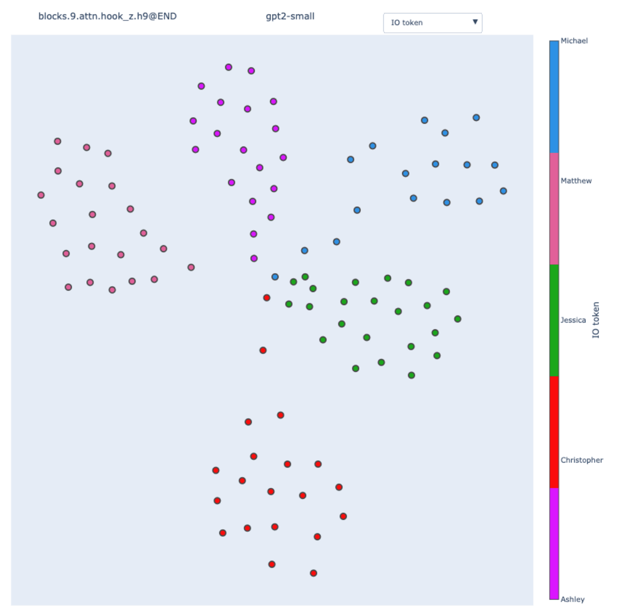
We observe clear clusters of inputs that perfectly correlates with the value of the IO token on these input sequences. It makes sense: swapping the input to the head doesn’t influence much the model output as long as the Name Mover returns the same value.
Nonetheless, the clustering is not perfect. In the center of the figure, we observe inputs that have different IO tokens but are close nonetheless. By coloring the node by the object (e.g. in the sentence from the circuit figure, the object is "drink"), we got:
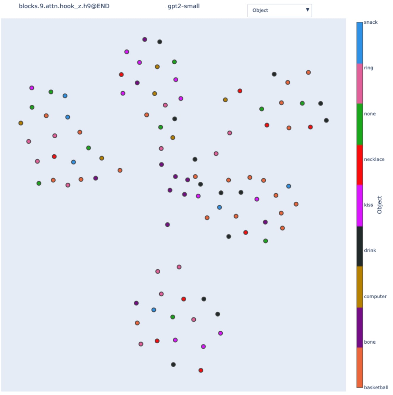
The inputs (dark purple points) in the center all involve the "bone" object. It's plausible that on these inputs, GPT2-small is not using the IOI heuristic strongly, but something that depends on the "bone" context. However, this observation is not true for all bone-related sentences as they are not all in the same place, so the story must be more complicated than that.
Takeaways
- Swap graphs are a natural extension of any input swap patching methods. They leverage all the possible input swap patching experiments given a dataset. They remove the burden of crafting in advance a hypothesis and alternative datasets, it instead uses the variety of features that exists inside a dataset. Nonetheless, it remains crucial to think about dataset design. In particular, to ensure a limited number of hypothesized feature values.
- Swap graphs output a firehose of bits [LW · GW] compared to hypothesis-driven patching. They expose potential outliers contradicting a hypothesis or alternative features that could matter for the component. This makes this technique well-suited for fast exploratory mechanistic interpretability.
- We demonstrate this in the following section by showing that swap graphs enabled a surprising discovery. We discovered heads in GPT2-small and a Mistral model that encodes the gender of the S token, despite this feature not being straightforwardly useful for the IOI task.
- They can show which features are encoded in the components’ output, even if we don’t know how they are computed. This makes this technique suitable to analyze large models. Swap graphs could provide an alternative to circuit-level analysis by giving a high-level, unsupervised description of the role of model components.
You can create your own swap graphs in this collab notebook!
A theoretical setting: reverse-engineering from causal interventions
Instead of directly trying to understand computation happening in neural networks, I found it useful to first consider an idealized reverse-engineering problem, generalizing the toy problem presented above. I think this theoretical setting contains important conceptual difficulties in understanding computation from causal intervention while removing the messiness from neural networks. In practice, I used it as a sandbox to refine my interpretation of swap graphs.
Problem setting
You have in front of you a processor. It’s an interconnected web of components, transistors, and memory cells that implements a program. You can control the input of the processor, and you can understand its output. However, you don’t know how to make sense of the intermediate electrical pulses that travel between components inside the processor.
What you can do instead is patch components. For this, 1) make two copies of the processor and run the copies on two different inputs 2) take a component from one copy and use it to replace its homolog on the other copy to create a “chimera processor” 3) Recompute the output after the patch and observe the result of the chimera processor.
How much of the program can you recover by running input swap patching experiments?
The naive interpretation of swap graphs
Here we'll focus on using swap graphs to answer this question and explore how much juice we can extract from them. In this setting, an edge is present in a swap graph iff , where denote the output of the chimera processor where the input to the component has been swapped for .
We call the program variable is encoding and the swap graph of on a dataset .
Claim 1: If two inputs and lead to the same value of in the program, they will be connected in . More generally, each possible value that can take on the dataset will create a clique[1] in the swap graph. This is saying that you can arbitrarily swap the input to as long as the value it stores stays the same.
One thing that would make swap graphs really cool is if the reciprocal to this claim was true. If we could decompose the network into cliques and know that all the inputs in each clique correspond to the same value of the underlying program variable. This would be an incredibly easy way to understand the role of ! This is what we implicitly did in the toy example above to guess that the teal component was encoding b%10. We call this the naive interpretation of swap graphs.
The naive interpretation of swap graphs: Swap graphs can be decomposed into disconnected cliques such that every edge is inside a clique. Each clique corresponds to a possible value of the program variable stored in the component.
As the name suggests, this interpretation is not true in general. First, swap graphs are not always decomposable into disconnected cliques where all edge is inside a clique. Second, cliques in a swap graph can contain pairs of input that lead to different values of program variables.
In the following paragraphs, we present counter-examples to the naive interpretation. We then used the counter-examples to state conditions that make the naive interpretation likely to be reasonable.
Counterexamples to the naive interpretation of swap graphs
I think that's a fun problem to think about counterexamples, feel free to stop here and think about them by yourself.
Swap graphs can contain strictly directed edges.
Take the program:
a,b
c = a*b
return c
You’re studying a component storing b. Here is a possible swap graph.
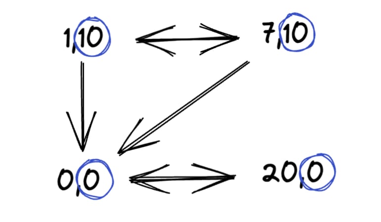
b input variable.If a=0 (bottom left corner), you can swap b with any value without changing the output, but the opposite is not true. So swap graphs are not made of bidirectional edges, and thus cannot be decomposed into cliques where every edge is inside a clique in the general case.
Okay, but in this case is easy to detect that something weird is going on because when a=0, the output doesn’t depend on b anymore. We could remove all inputs that can be swapped arbitrarily without influencing the output i.e. the edge exists for every .
Unfortunately, this is not enough.
Swap graphs can contain strictly directed edges even when filtering for dependency.
a,b
return a%b
Here is a swap graph for a component storing a on a dataset of 3 samples.
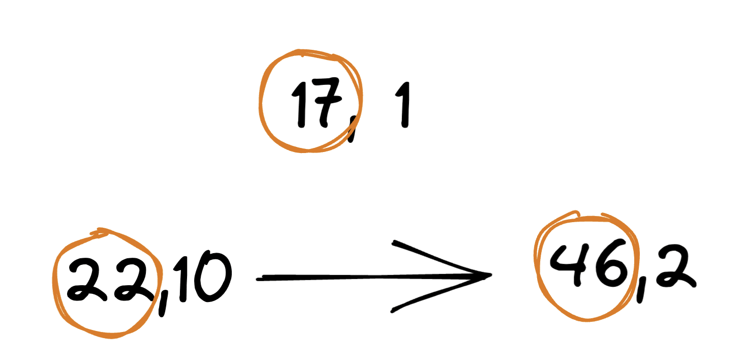
a input variable.No need to filter any input because of independency as there is no edge from or to (a=17, b=1).
We still have a strictly directed edge because but .
Okay, but when we have a clique where all elements are bidirectionally connected, then we can interpret this as a sign that the underlying variable has the same value, right?
No.
Cliques in swap graphs don’t map to variable values in the program.
a,b
c = a+b
return c%2
A swap graph for a component storing c:

Because the output can only be 1 or 0, there is a lot of wiggle room. As long as the output has the same parity, inputs that lead to these various values will be connected to the swap graphs. The final modulo 2 is washing away a lot of the information contained in the intermediate variables, creating edges "by coincidence".
Takeaways to interpret swap graphs in practice
Takeaways from the counterexamples
From these counterexamples, we can take away principles that make the naive interpretation break. The following points are about known failure modes, not comprehensive rules.
Thus, we are more confident in the naive interpretation:
- When the output always depends on the component you’re investigating.
- When the intermediate variables and the output contains a lot of information such that it’s unlikely to be the same by coincidence.
These principles can be applied to empirical swap graphs on neural network components. For instance, a practical way to implement the second point is to measure the full output probability distribution and not just a few logits to catch any deviation (but this also changes the scope of the behavior you’re studying as you're not always interested in explaining the full distribution, there is a tradeoff here).
A (hand-wavy) frequency argument to design datasets that favor the naive interpretation
We can also rely on a frequency argument to interpret swap graphs, again using a simple model. We can see a swap graph as being made of cliques (that we expect because of Claim 1.) plus additional edges coming from swaps that did not change the output of the model for other reasons than keeping the underlying variable constant. Here, we model the additional edges as noise.
Then, we can choose to design a dataset such that the number of edges from the cliques is expected to be larger than the noise. For the cliques to be large, their number should be small. I.e. the number of possible values of the abstract variable should be small. Of course, it still needs to be greater than 1, else the whole graph is a clique.
To enforce this regime, we can make hypotheses about likely variables a component can encode and reduce the number of values they can take on the dataset. This is easier than designing a hypothesis about a specific variable a component can take. If you control the process by which the dataset is created (e.g. by relying on templates with placeholders), it is easy to restrain the number of values taken by all your variables. Swap graphs can then tell you which of the many candidate variables a component is encoding, without having to test them one by one. Moreover, some variables naturally take a limited number of values (e.g. the gender of a character).
The empirical naive interpretation
Here is the summary of the points made in this section. This form the lens through which we'll interpret the swap graph in practice:
The empirical naive interpretation of swap graphs: When a swap graph can be decomposed into separable communities, we interpret each community as a possible value of an abstract variable that the component is encoding when run on this dataset. We are more confident in this interpretation when we measure a rich output of the model, and when the number of possible values the abstract variable can take is low. Such an abstract variable, when it exists, is interpreted as an approximation of the role played by a component.
Extension of the theoretical setting
Despite all these considerations, we don't have a guarantee that our component can cleanly be modeled as "storing a simple variable that will be read by later layers". Models are messy and components can play several roles at the same time by representing features in different directions, or even in superposition. Here is a list of possible extensions to better model the peculiarities of neural network representations and design more precise experimental techniques.
- Components storing different variables. So far, we considered components as atomic registers that can store bits of at most one variable. What if instead components are memory blocks that could host several variables at the same time? This would be a more accurate modeling of what happens when we compute the swap graph of a large part of an LM such as an MLP block.
- Continuous variables. Most of the arguments we made so far would break when the abstract variable a component is encoding can take continuous values. In this case, we could think about leveraging close but not exact matches in the values, under some continuity assumption about the model.
- Advanced patching. We considered so far a simple experimental primitive that swap inputs to a component. However, techniques such as path patching enable more precise intervention, allowing to patch only specific paths in the computational graph.
- Such interventions are likely to help when components can store different variables. A given component can be interpreted differently along different paths, such as patching only one path would fall back to the monosemantic case.
Comparative LM anatomy: studying the IOI task in multibillion parameter models
Manual study of IOI on GPT2-small
Technical implementation
Since we have extensive information about IOI in GPT2-small, we chose this task to validate swap graphs and their interpretation.
Metric choice. However, because we used KL divergence as our metric, the scope of the behavior we’re investigating is different than what has been studied in the IOI paper that focused on logit differences. Here we aim at understanding the full probability distribution, not just why the IO token is predicted more strongly than the S token.
We made this choice of metric i) to be able to gather data that would generalize to other tasks where logit difference can't be used but KL divergence can ii) because of our empirical naive interpretation, we are more confident in interpreting swap graphs that measure the rich output of the model. We nonetheless validate some of our findings on GPT2-small by running swap graphs with logit differences in Appendix.
Dataset. For all the experiments presented in this post, except when mentioned explicitly, we used a modified version of the IOI dataset generation introduced in the IOI paper where we restricted the number of possible names to 5. We made this choice because we expected the various names to be important features and we were motivated to make the naive interpretation more likely.
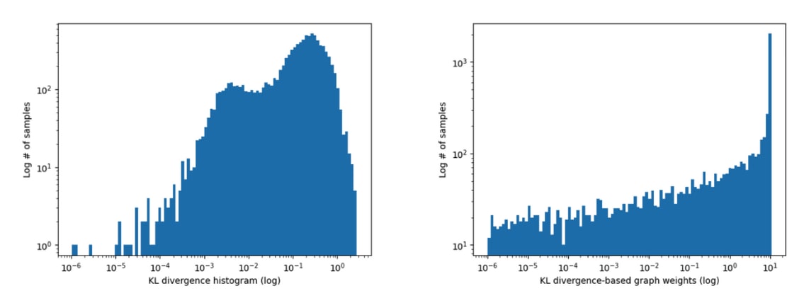
Gaussian kernel. Network analyses and visualization are easier when the weights of the edges represent similarities or attraction forces, rather than distance. To turn the raw weights of KL divergence into graph weights, we used a Gaussian kernel with a standard deviation equal to the 25th percentile of the raw weight distribution. This choice is somewhat arbitrary, but we found that the structure of the graph is not highly sensitive to the choice of metric or kernel function.
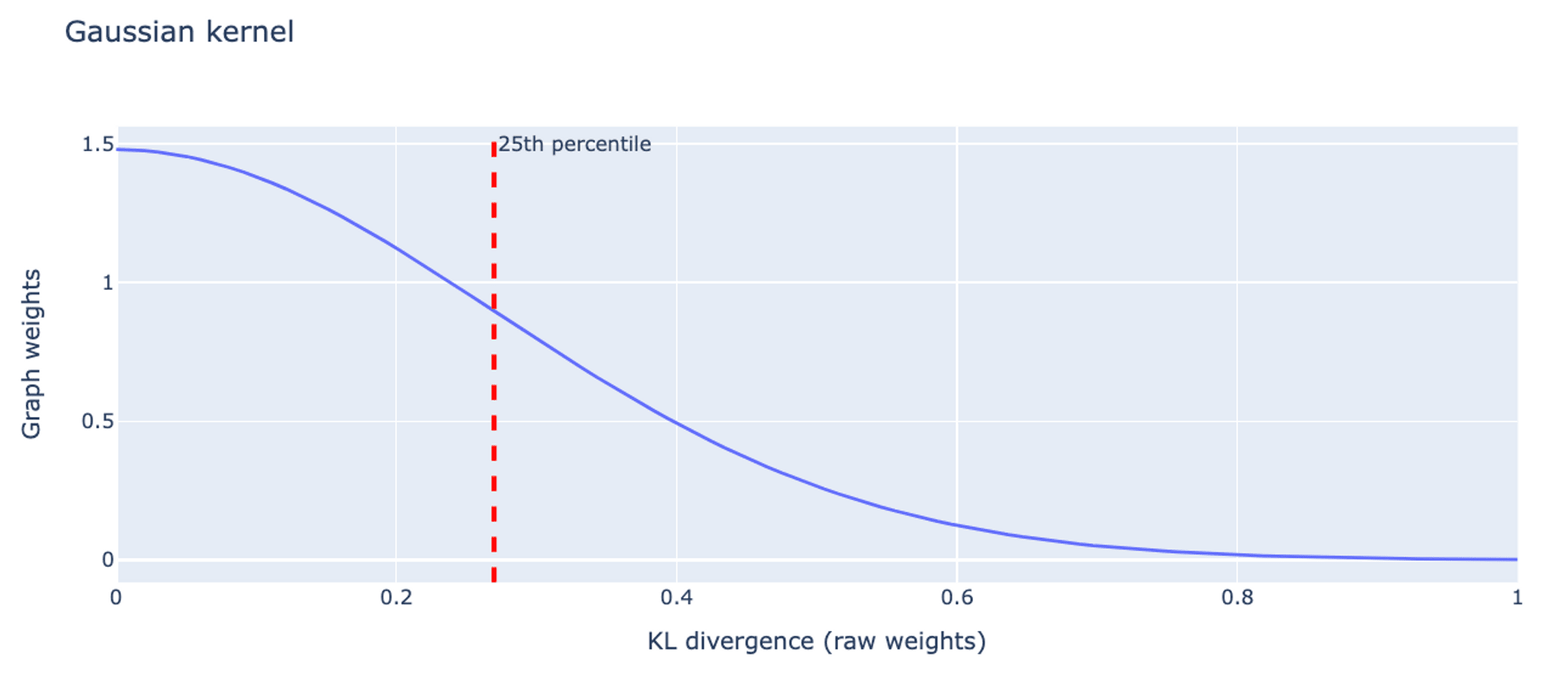
Here are on the left the distribution of the swap graph of 9.9 on IOI raw weights (the KL divergence scores) and on the right the graph weights after applying the Gaussian kernel.
Swap graphs deeper into the IOI circuit
Name Mover's queries.
In the previous experimental results, we investigated the swap graphs of the output of 9.9. We can do the same by input swap patching its queries instead.
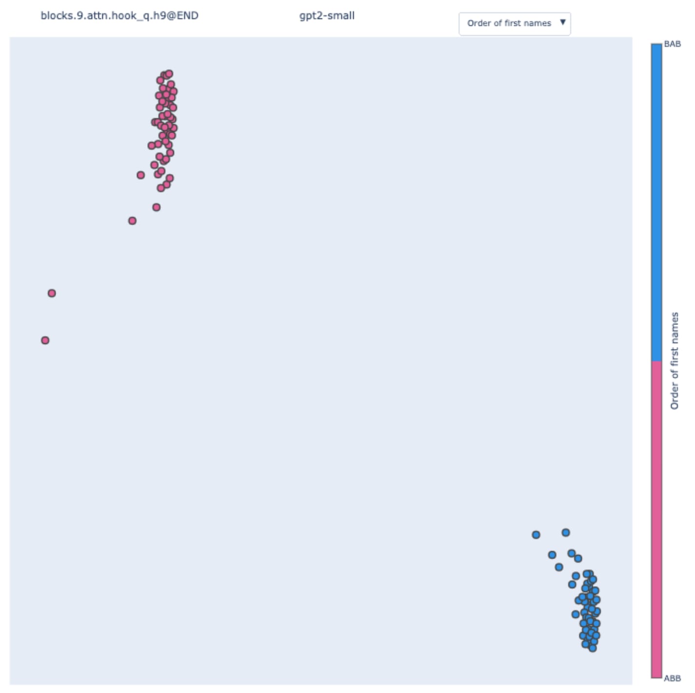
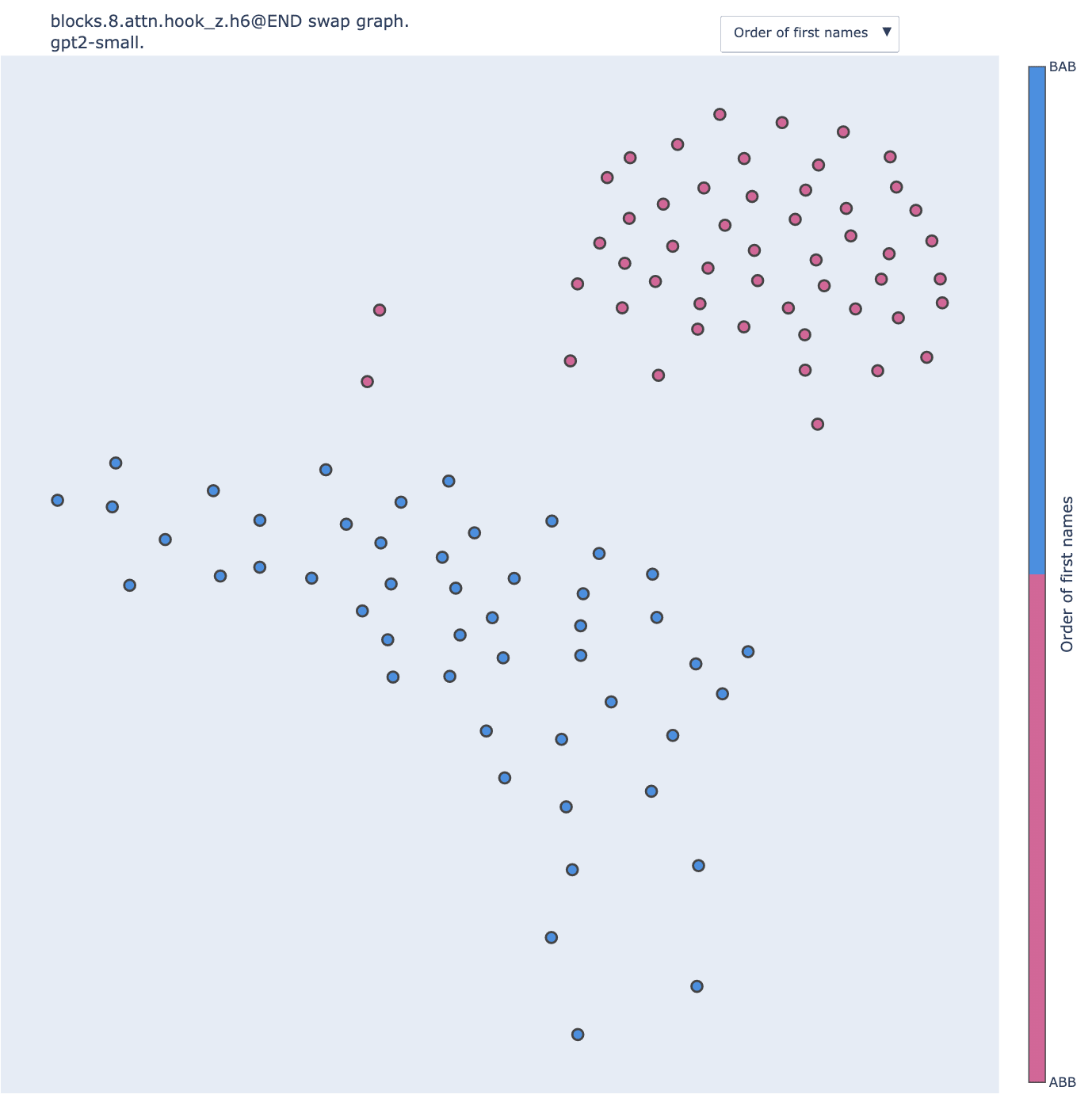
Here, the clusters correspond to the order of the first name, i.e. if the template is of the type ABB or BAB. “Alice and Bob went to the store. Bob …” is of the template type ABB “Bob and Alice went to the store. Bob …” is BAB.
This is coherent with the results presented in Appendix A of the IOI paper (that was done using hypothesis-driven patching). Name Movers rely on S-Inhibition Heads through query composition to compute their attention specific to IO. S-Inhibition Heads are sending information about the position of the S1 token and its value, with the first piece of information having more weight than the second. They are saying to Name Movers “avoid paying attention to the second name in context” more than “avoid paying attention to the token ‘Bob’“. We called these two effects, position signal, and token signal respectively.
What we observe here is that the value of the position signal perfectly correlates with the two clusters present in the swap graph. Hence 9.9's queries are encoding the template type.
S-Inhibition heads.
We know that the position signal originates from S-Inhibition heads. Let's track it down!
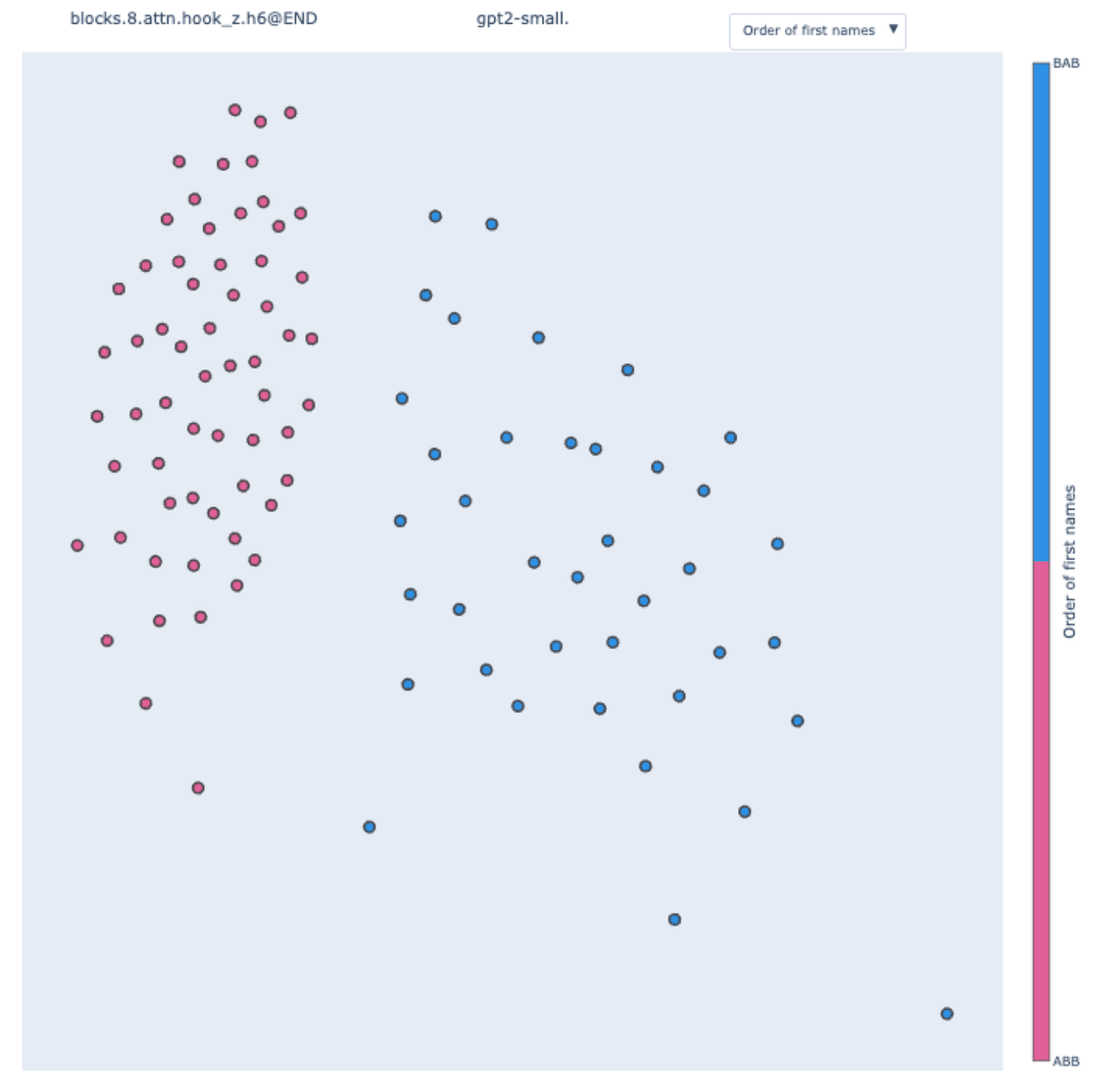
The two clusters are present and again perfectly correlate with the template type.
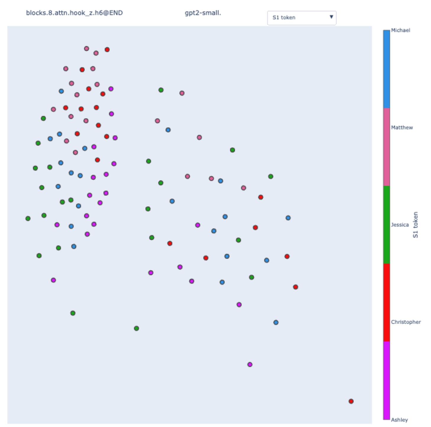
When coloring by the value of the subject token, we observe partial sub-clusters inside the main clusters. To validate this observation, we can "zoom in" on a particular cluster by creating an IOI dataset with only the ABB template type.
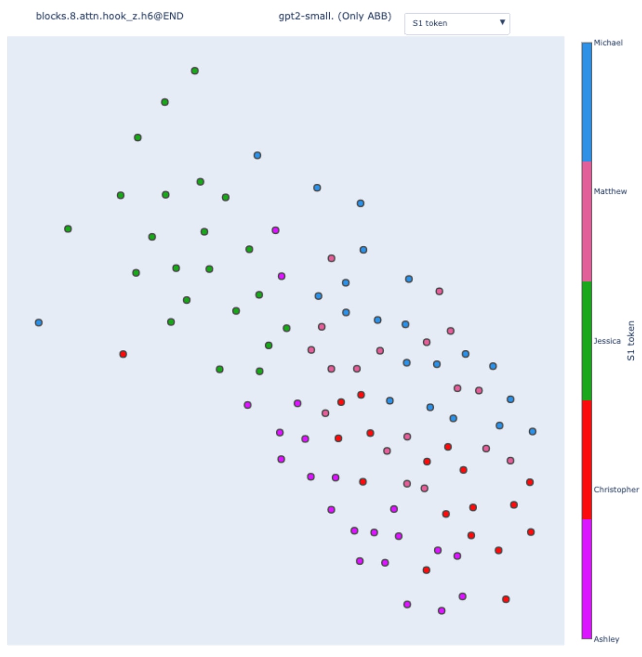
This validates the observation: once the template type is fixed, the second most important feature is the value of the subject token. This is coherent with the existence of the position and token signal, and by analyzing the hierarchal order of the feature in the swap graph, we recover their relative importance.
This is an example of disentangling two variables encoded by the same component.
Going deeper: duplicate token heads and induction heads.
We can continue our journey in the depth of the IOI circuit and track the origin of the position and token signal even further. Here is the IOI circuit again.

Here is the induction head 5.5 at the S2 position:
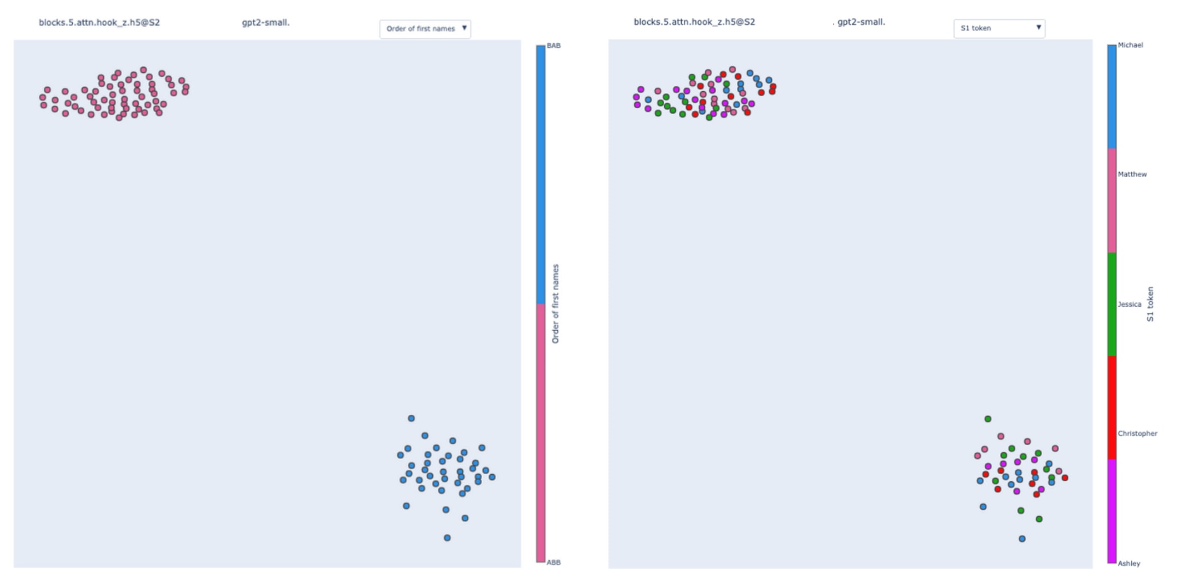
One weak induction head 5.9:
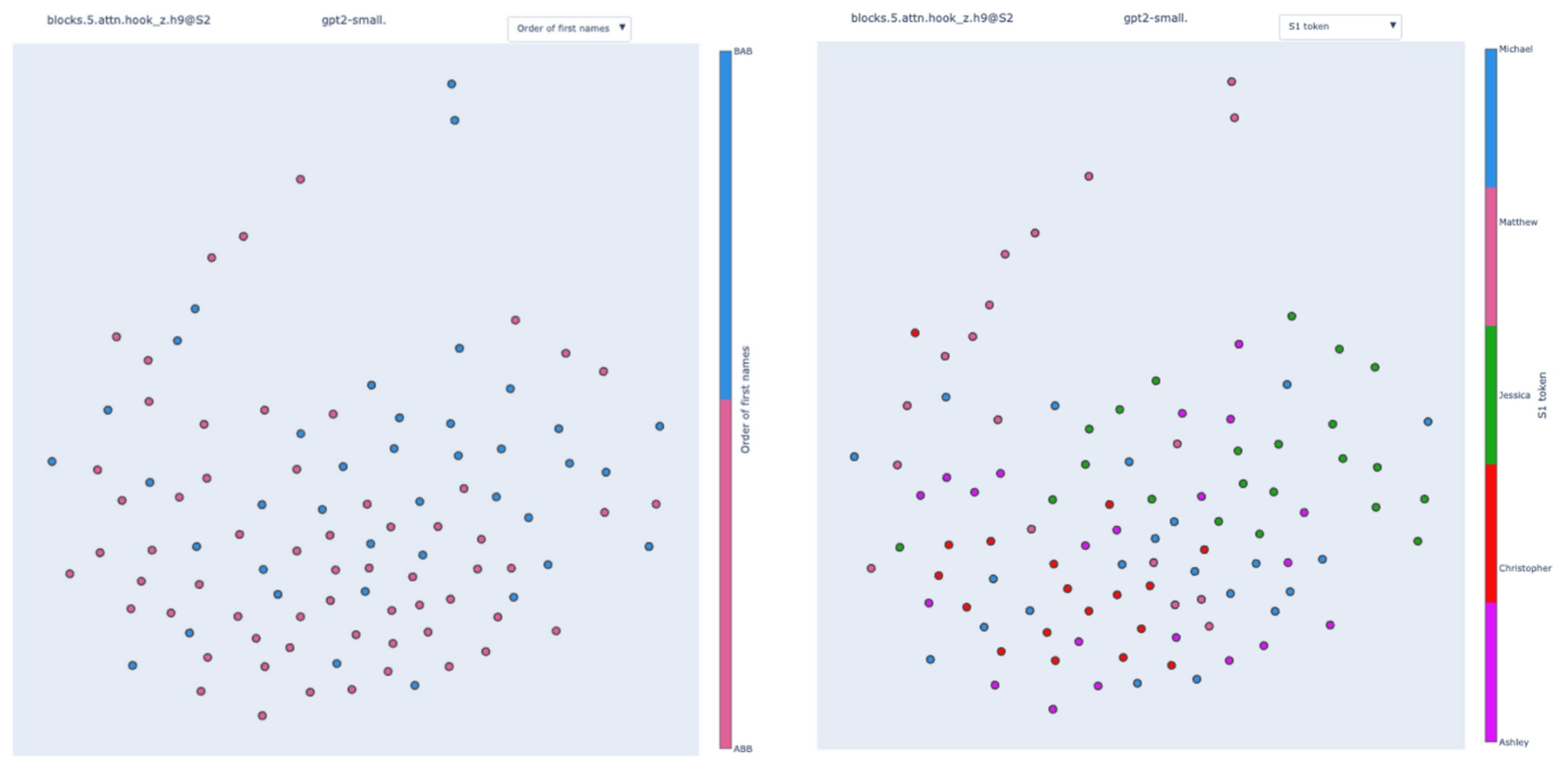
That’s a good example of a weak/absent pattern in a swap graph. I’m uncomfortable interpreting any structure from these plots except that there doesn't seem to be any interpretable structure.
Here is the duplicate token head 3.0:
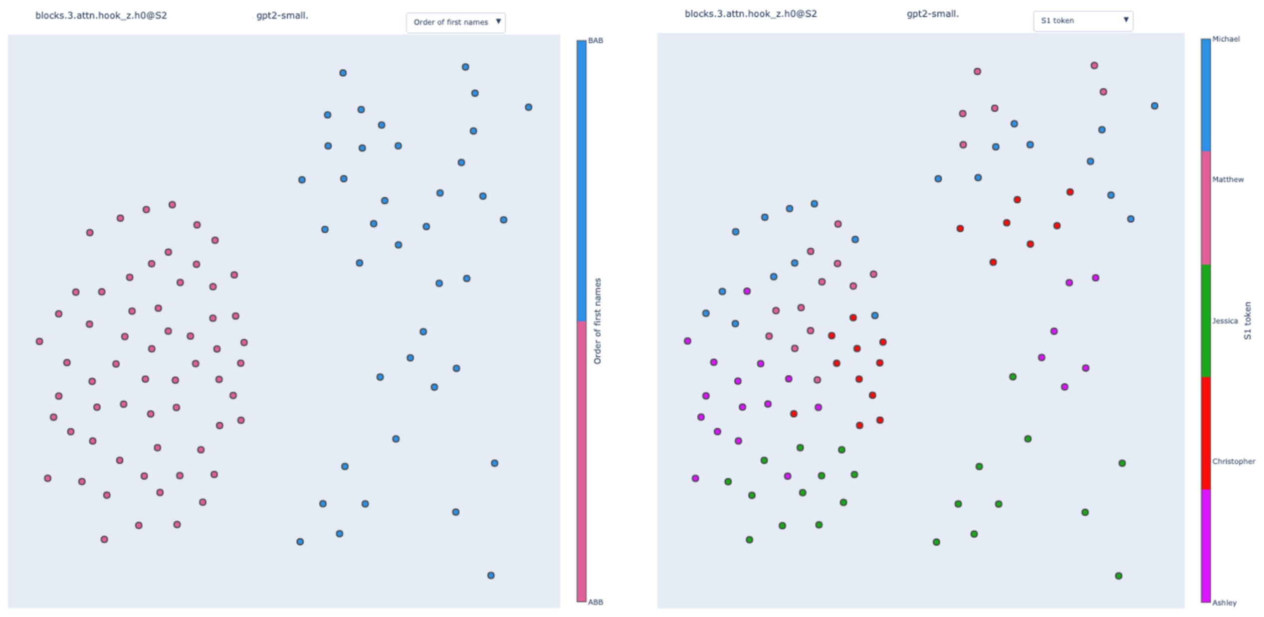
Surprising results in a Mistral model and GPT2-small: gendered S-Inhibition heads.
For now, we’ve only been confirming results already described in the IOI paper. But this new technique enabled us to make surprising discoveries.
We tried to reproduce the study on a mistral model with the same architecture as GPT2-small (the model is called "battlestar"). Through path patching, we found the structural equivalent of Name Movers (heads directly influencing the logits) and S-inhibition heads (heads influencing Name Movers).
When we computed the swap graph of 8.3 at the END position, a structural analog of the S-Inhibition heads, we observed:
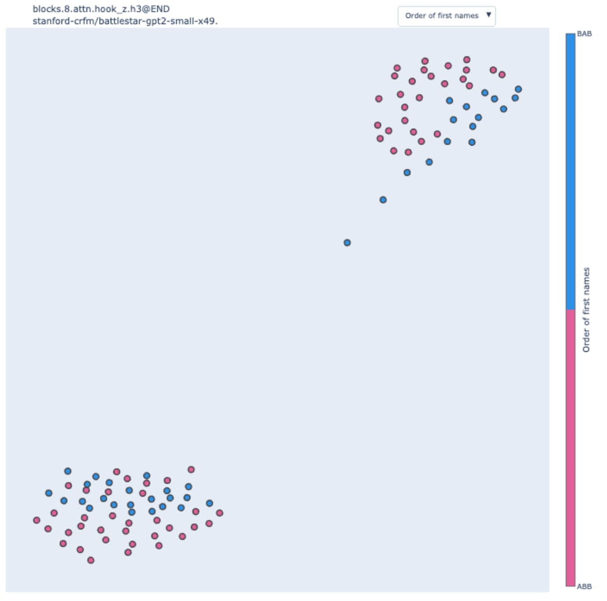
We observe two clear clusters, but the order of the name is only of secondary importance. By looking at the sentences in each cluster, we discovered that they perfectly correlated with the gender of the subject.
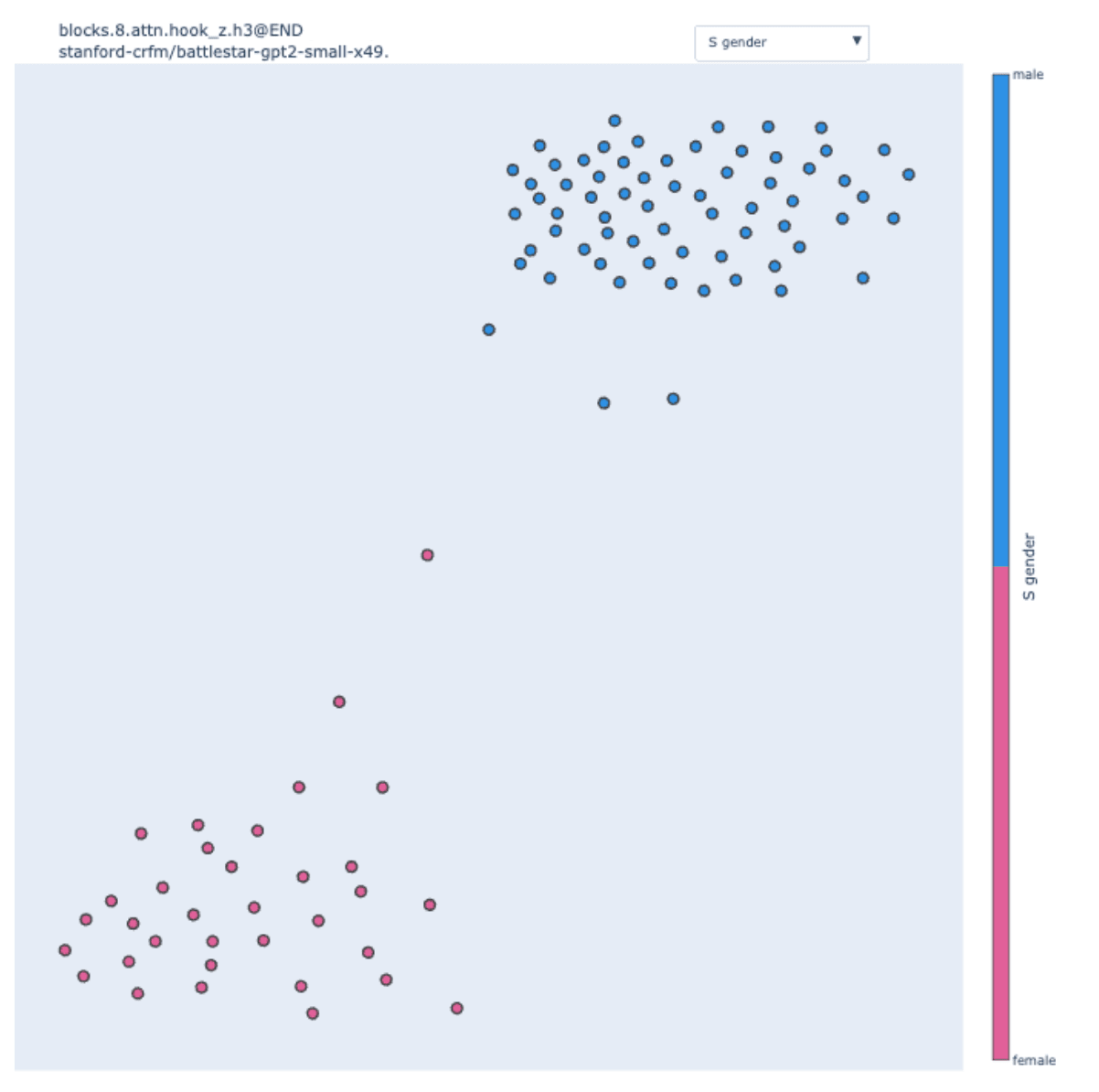
This result holds when allowing more than 5 possible names. We used genderize.io to attribute a gender to 88 different names to color the figure above.
By looking back at GPT2-small and running pathing networks for more heads, we discovered that 9.7 (a weak Backup Name Mover head) was also, in fact, a gender head.
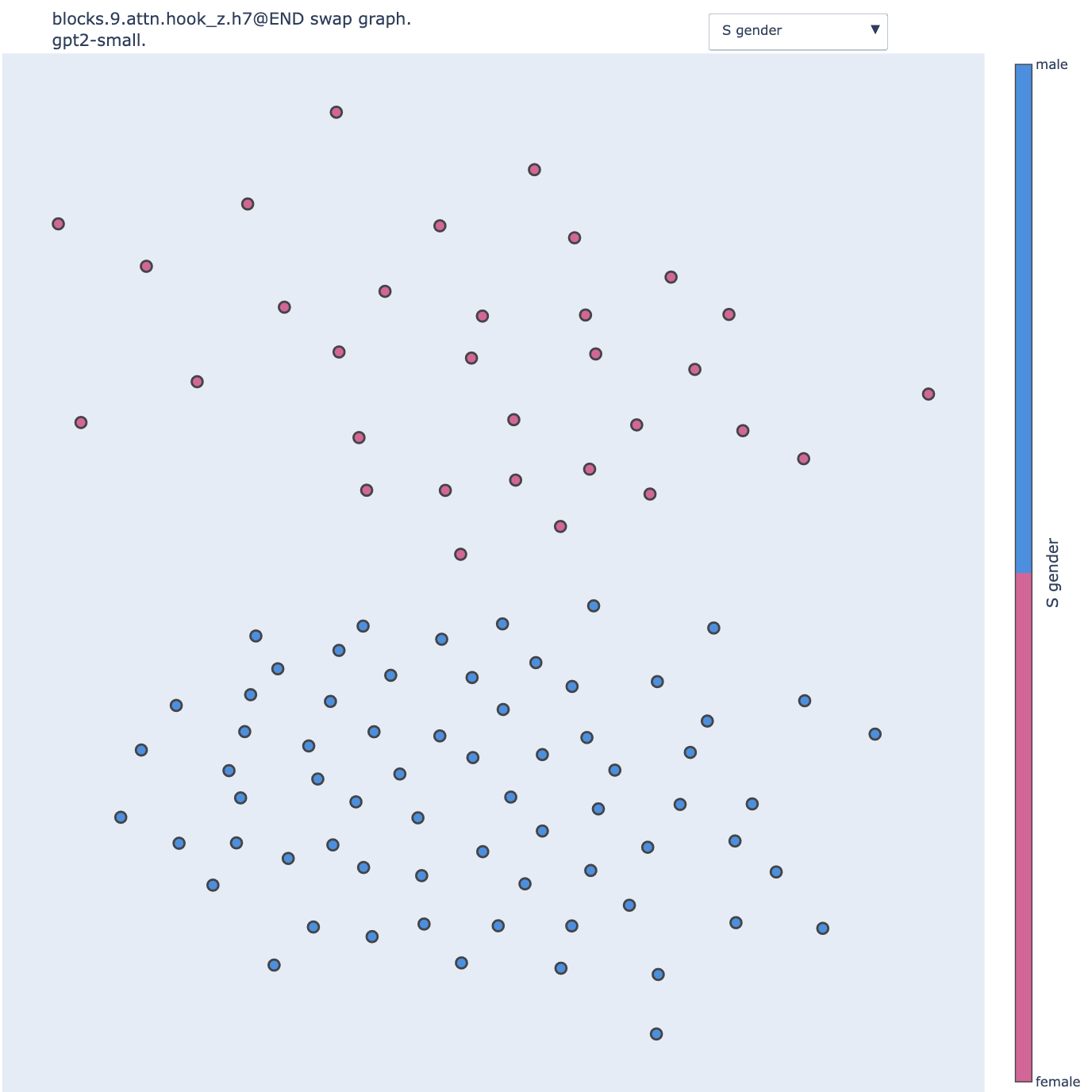
Despite being part of the IOI circuit, this head is in fact quite poorly characterized in the paper because of its weak importance. This is thus not particularly surprising that the IOI paper missed important parts of its role. Similarly, 8.3 in the mistral model is also not the most crucial head for the model computation.
I don’t have a good understanding of how gender information is used. There is no reason for it to be used a priori, and this fact would have been hard to find using hypothesis-driven patching. I was able to discover it because I observed two clear clusters that didn’t map to the features I hypothesized at the time.
Scaling to larger models
Community detection. To scale to a bigger model, we automated the process that we did manually so far: eyeballing clusters and how they match different coloring schemes. We start by detecting communities in the swap graph with the Louvain method. Then, we compute their adjusted Rand index with values taken by hypothesized abstract variables (i.e. discrete functions of the input like the IO token). This index is a measure of similarity between partitions of a set, in this case, the partition outputted by the community detection and the partition induced by the hypothesized variable. The index is adjusted, meaning that a score of zero is what we expect for two random, independent partitions.
Semantic maps. To evaluate swap graphs on larger models, we run them on every component (attention head and MLP block) at the END position on the IOI dataset and compute their communities.
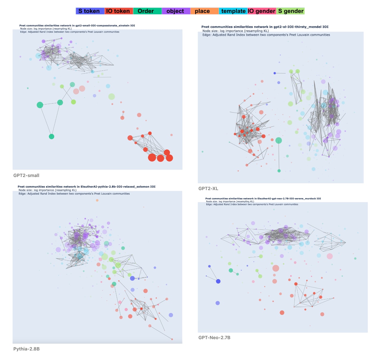
From there, we introduce a new visualization technique called a semantic map to have a comprehensive view of the role of every component in a single figure. A semantic map is an undirected, weighted, complete graph where nodes are the model components , and the weight of the edge is defined by the adjusted Rand index between the Louvain communities of and .
Intuitively, the more connected two components are in the semantic map, the more similar the abstract variable they encode (to the extent they encode one).
We used four models for our comparative analysis: GPT2-small, GPT2-XL, Pythia-2.8B, and GPT-Neo-2.7B.
Again, we used force-directed graph drawing to visualize the graphs. We used the following visualization scheme:
- Color: the feature with the highest adjusted Rand score with the Louvain communities (among a list of 8 features I manually defined).
- The opacity is proportional to the value of the highest adjusted Rand index (with a minimal value to make all nodes visible).
- Size: log of the importance of the component as measured by average KL divergence on resampling ablation. This is also the average weight in the swap graph of the component.
- The edges are shown when the adjusted Rand index is greater than 0.5.
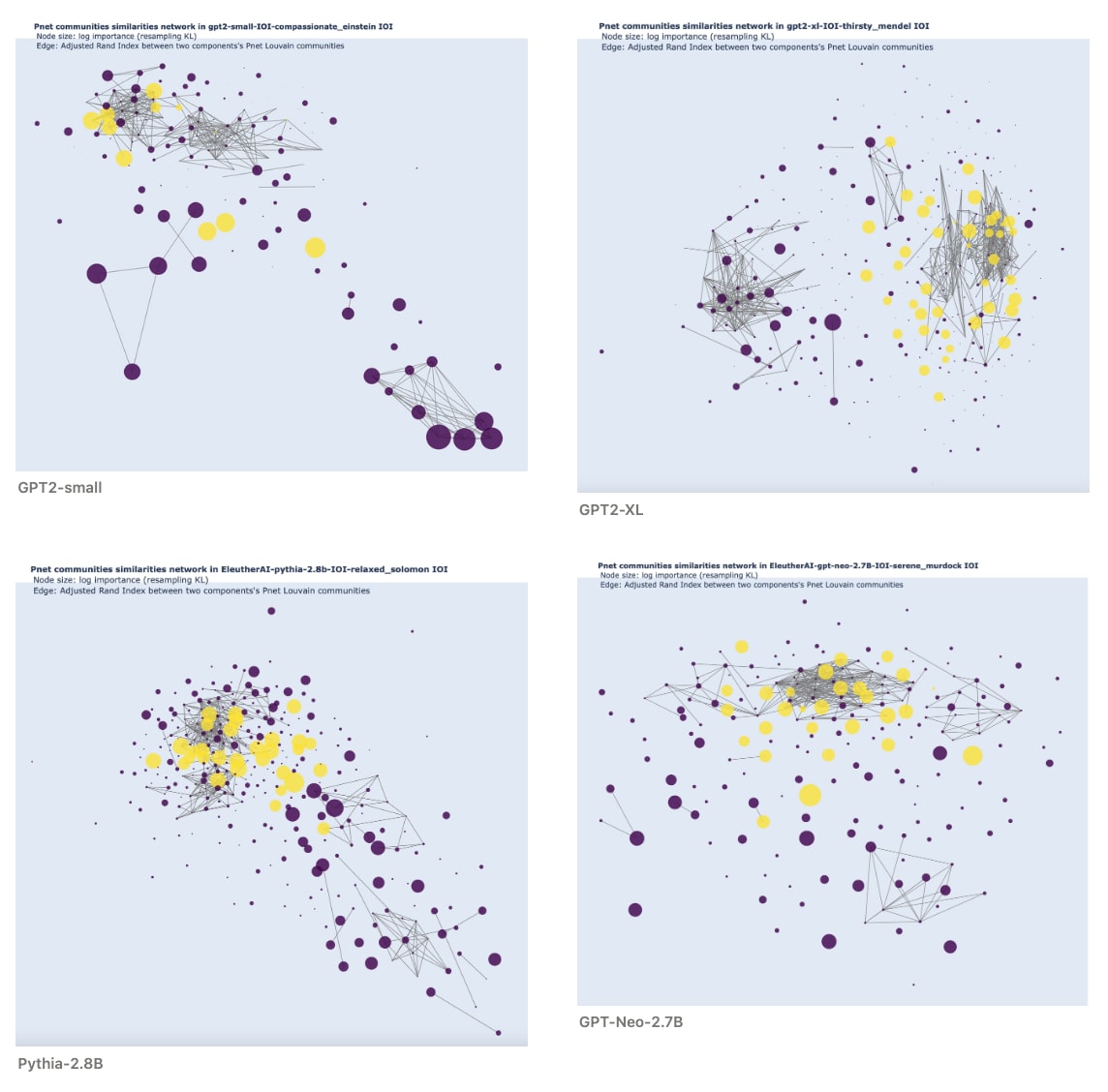
Here are the same graphs, colored by component type: yellow for MLP, and dark blue for attention heads.
You can find all the plots as interactive HTML, with more coloring (by layers, by feature, etc), in this drive folder.
Observations/comments
I’ll use “encode” as a way to mean “whose swap graphs’ Louvain communities on the IOI dataset have high adjusted Rand index with”.
- MLP blocks seem to have consistent communities, but they don’t strongly correlate with any known feature. Most of them appear transparent and slightly correlated with the object value. But the correlation between them is much higher (adjusted Rand index >0.5) than the correlation with the object value (adjusted Rand index 0.1-0.25). Nonetheless, they also are not well clustered (modularity < 0.3). I’m thus uncertain to interpret too much this information.
- Inspecting manually some of them revealed that they seem to be sensitive to the end of the sentence. I.e. whether the sentence ends in "said to", "give {OBJECT} to" or "give it to".
- In the four models, we identify a community of attention heads that encodes the IO token. They are clearest in the GPT2 models and overlap with the Name Movers found in the IOI circuit for GPT2-small. I hypothesized that in larger models, they are the homolog of Name Movers in GPT2-small.
- In between the communities of Name Movers-like and the majority of MLPs, we find subgroups of heads that encode the ABB/BAB template type, the S gender, and the S value. I hypothesized that they are the homolog of S-Inhibition heads: they gather information about the S subject (its position in dark green, gender in light green, the token value in dark blue) and transmit it to steer the attention of the Name Movers homolog.
- The two biggest models (Neo and Pythia) have more transparent nodes. These components are not well described by any of the 8 candidate features. This makes them less well described using swap graphs and manually defined features, but many of the adjusted Rand indices are significantly above zero so we are not interpreting noise.
- At a high level, the four model looks surprisingly similar given this visualization. This gives hope to designing high-level explanations that can transfer through scale and models.
Semantic maps of queries.
To build swap graphs, instead of patching the output of the component, we can patch the queries input to the attention head. Then, we can compute semantic maps on the queries (and restrict the components to attention heads). This time we only ran it on the 10% of the component with the most important queries. You can find all the plots in the drive folder.
Validation of swap graphs in larger models
Considering the low adjusted Rand indices between swap graph communities and manually created input features on larger models compared to GPT-2 small, it's natural to question the significance of the high-level structures we observe. In practice, most swap graphs are not cleanly separable into tightly connected communities.
To validate that swap graphs enable us to make predictions about the model mechanism, we designed two sets of downstream experiments leveraging the information contained in the Louvain communities. First, we checked that we can swap the input inside communities without impacting the output of the model (that's a kind of causal scrubbing experiment). Second, we created targeted rewrites of specific components by swapping their input across communities to trigger a precise model behavior.
Causal Scrubbing: resampling inside the communities
A first sanity check to ensure that we can naively interpret swap graphs and their communities is to resample the inputs inside the Louvain communities. If each input inside a community lead to the component representing the same value, we can swap it for an arbitrary input from this same community. The value represented should stay the same, and thus the output of the model should not change much.
Resampling all the components at once is not a really interesting experiment to run. If the model uses complicated circuitry before returning its answer, such that the output only depends on the last part of the circuit, then resampling the input to all the components is equivalent to resampling the last part of the circuit. We will never test how much we can preserve the structure of the intermediate nodes.
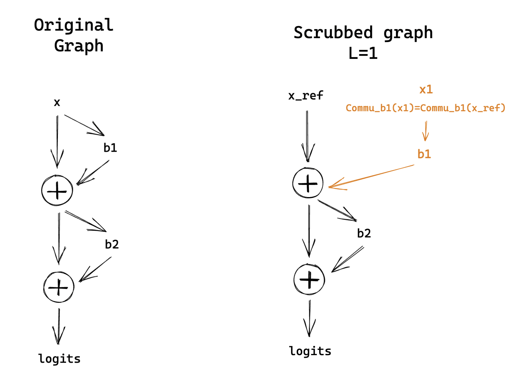
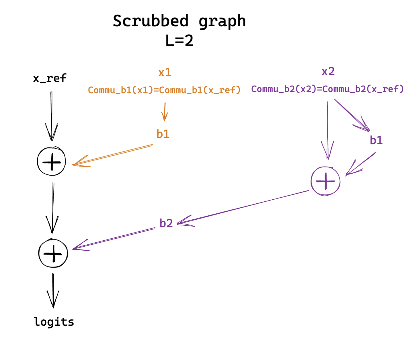
To limit this, we run resampling by communities of all components before the layer for all layer . This means that we also measure if the model can compute the end of its forward pass and return meaningful output despite all the early components being run on resampled inputs.
This is a particular kind of causal scrubbing experiment where we don’t fully treeify our model and define equivalence classes for resampling. More precisely, the scrubbed computational graphs on a toy example for different values of looks like this:
Scrubbing baselines.
To compare the performance of the causal scrubbing from swap graphs, we introduce two other methods to partition the inputs.
- Random communities. Each input sequence gets randomly attributed a number between and . The number represents the community it’s part of. Each component gets an independent random partition using this method.
- Clustering on the activation vectors. Instead of running patching interventions to compare how two inputs , influence a component , we could directly compare the activation vectors of on and . This is a much cheaper operation to run. More generally, we run hierarchical clustering on the set using the Ward’s method.
Each of the three methods takes hyperparameters that control their tendencies to favor small (but numerous) communities, or large (and less numerous): for random partitions, the resolution in the Louvain algorithm (the default value we used so far is 1.), and the linkage threshold for Ward’s method.
Of course, we expect that the smaller the communities, the less destructive the resampling would be. In the limit, each community contains a single element (e.g. random communities with ), and the resampling has no effect.
Comparing partitions
To fairly compare the results of the three methods, we need to evaluate the size of the partitions they return, i.e. where they lie between one set per sample and one big set containing all the samples. To this end, we used two metrics:
- The average community size (average over communities and components). In the figure below, we show the relative size compared to the full dataset of size 100 samples.
- The average entropy of the resampling operation (average over components).
- For each component, the resampling operation can be seen as drawing uniformly at random a permutation from a set of permutations where only elements inside the community can be permuted, and applying to the dataset as input to . is made of the composition of fully random permutations for each community. The entropy of this distribution of permutation is thus where is a community and its size.
For each method, we chose a set of 5 hyperparameters such that the partition metrics span similar ranges. Each lie color corresponds to roughly the same average resampling entropy and community size.
Experiment results.
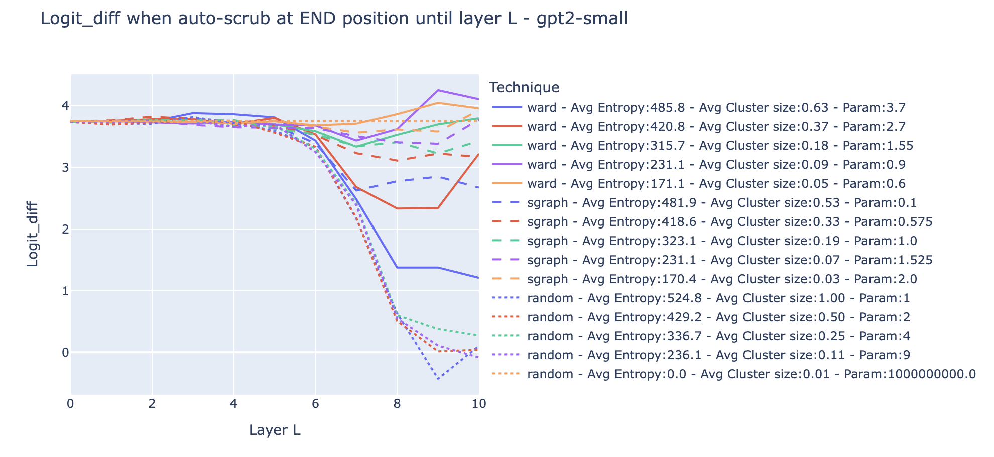
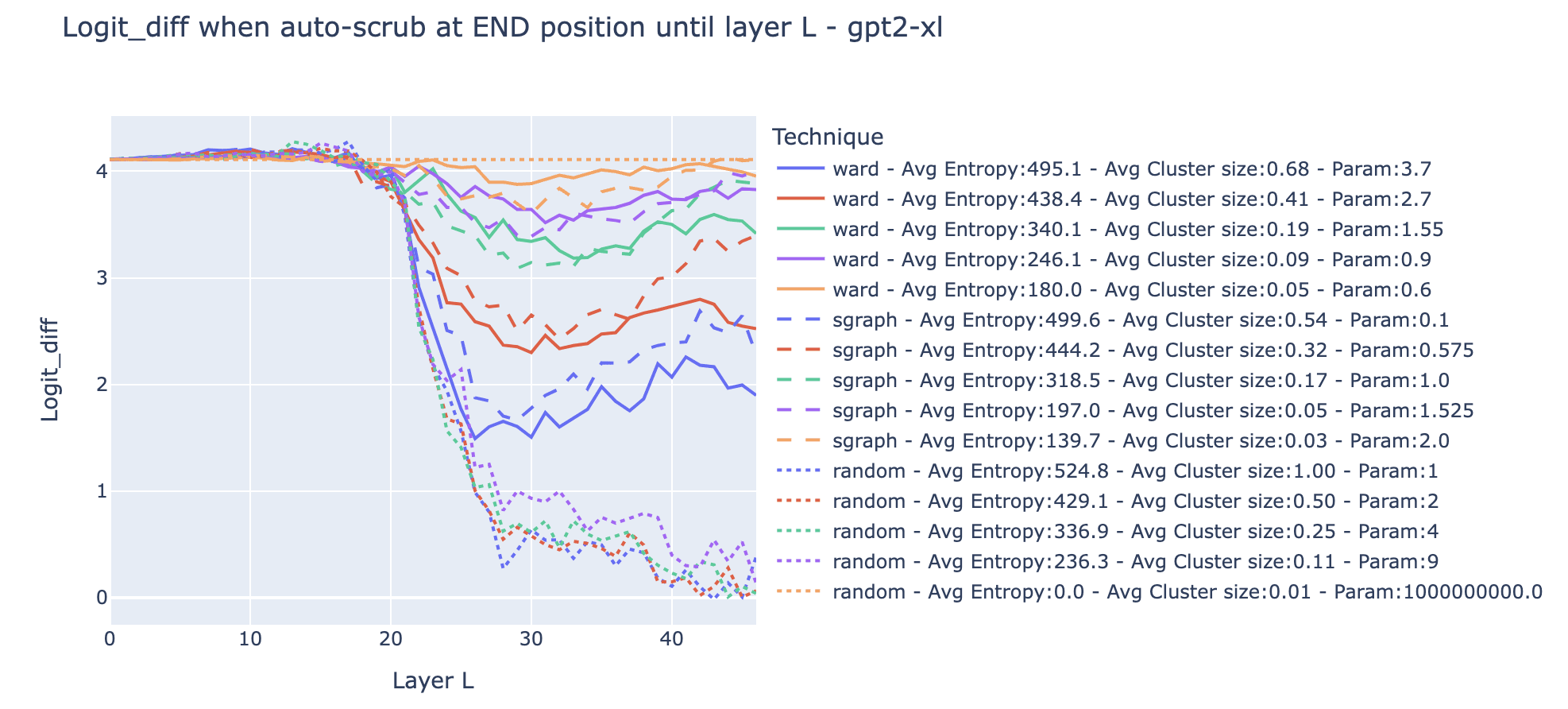
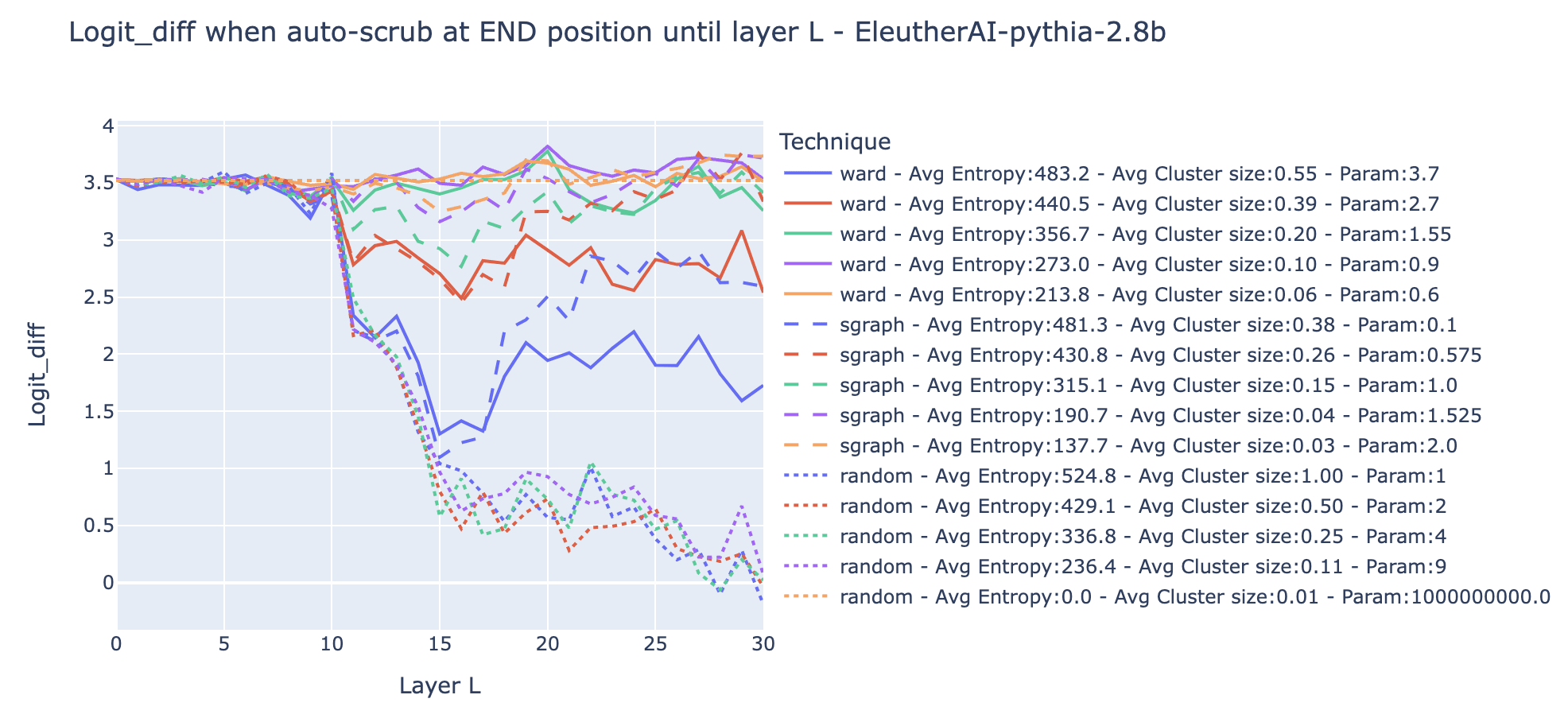
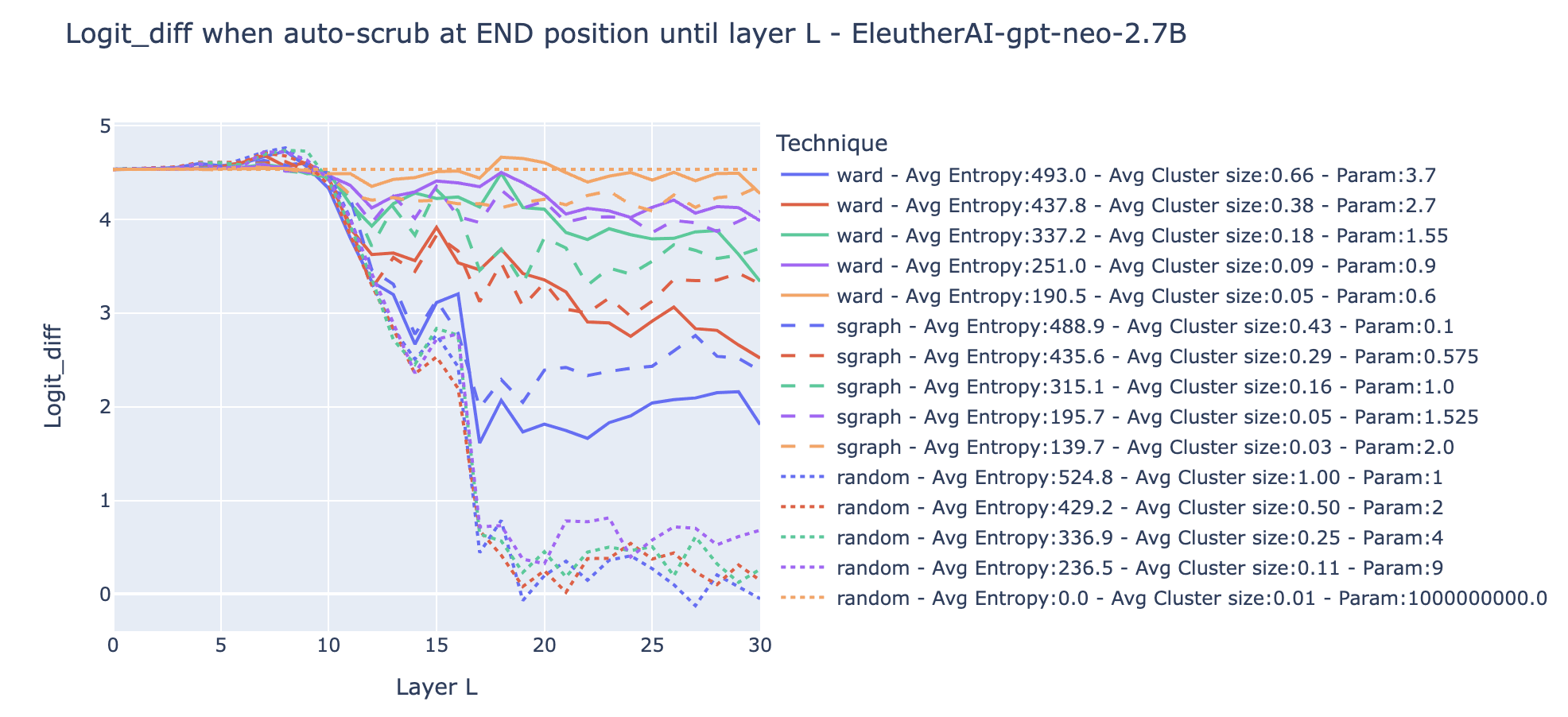
The results for the IO and S probability can be found in the drive folder.
Observations/comments
- The dotted orange line is the random partition with such that each sample is its own community: average entropy is 0, and the average cluster size is 1. That’s the case where there is no resampling, so the experimental result is the same no matter the layer (this is a good verification that there is no obvious bug!).
- Most of the curves are clearly not monotonic (e.g. dashed and solid blue curves). For both the clustering on the activation vectors and swap graphs, scrubbing all layers until the mid-layer led to a lower logit difference than scrubbing all the layers. We interpret this as meaning that it's easier to preserve the structure by scrubbing the last components of the circuit (e.g. the equivalent of Name Movers) than scrubbing the components in the middle of the circuit when the last components are recomputed.
- Clusters from swap graphs lead to less destructive resampling on average than clusters computed from activation alone when controlling for the entropy of the resampling, in the regime where the entropy is high (blue and red line). When the entropy is low and thus the average cluster size low (green, purple, and orange lines), both clusters from swap graphs and activations vectors perform roughly equally well.
- This suggests that swap graphs are a useful technique to find partitions of the inputs that preserve the internal function of the model. However, it comes at the cost of more compute. To determine more precisely how much clustering on swap graphs enables better causal scrubbing experiments, we should further treeify the model and recursively resample the inputs.
- The dashed green line (Swap graphs with a resolution of 1.) is what we’ve been using so far. It seems to be a good tradeoff between the entropy of the distribution and the preservation of the structure.
This is a reassuring validation that the naive interpretation seems to make sense empirically. In some way, this is the minimal test that swap graphs and our interpretation are required to pass to be willing to give weight to them.
Targeted rewriting: patching across communities
In the previous experiments, we validated that the Louvain communities correspond to sets of inputs invariant by swap. But we did not make use of the knowledge we gained with the semantic maps. This is what this section is about.
If we claim to understand the variables stored in various components, we could also imagine how changing the variable stored in a set of components will affect the rest of the layers and eventually the output of the model. We can even imagine how to change the model to put it in a configuration we never observed before (e.g. implanting a jellyfish gene in the DNA of a rabbit). If we’re able to predict the results of such experiments, this is a good validation of our understanding.
We call such experiments that make a model behave outside of its normal regime in a predictable way targetted rewrites. In that, they differ from causal scrubbing which measures how much the model behavior is preserved when the internal distribution respect a given hypothesis.
Targetted rewrite on Name Movers
We did not conduct any circuit analysis of the kind performed in the IOI paper on the larger models. Nonetheless, in this section, I'll draw parallels between components from the IOI circuit and components from larger models using information from swap graphs alone. More work is needed to know how much these parallels make sense. For now, you can see them as a way to touch reality quickly to see if I can modify the model behavior by swapping inputs across communities for specific components -- an essential part of the naive interpretation view.
Similarly to the behavioral definition of induction head [LW · GW], I define a continuous definition of extended name mover that relies on high-level observation about the head and not on a precise mechanism. An attention head in a TLM is an extended name mover if
- Its attention probability from the END to the IO token is in the th percentile among all components at the END position and
- Its adjusted Rand index between the Louvain communities of its swap graph and the IO token is also in the th percentile among components.
The intuition behind this is that we want to find heads copying the IO token. The first point is a proxy for checking that they attend back to it (instead of e.g. repeating the value of the IO token sent from earlier layers), and the second point is checking that the primary variable that explains how they influence the output when swapping inputs is the value of the IO token.
Once we identified the extended name mover, we change their input such that they are outputting a name that is not the indirect object. The goal is to measure if this translates in the model outputting the alternative name instead of the indirect object.
More precisely, we chose an arbitrary rotating permutation of the 5 possible IO tokens and retargeted all extended name movers to output instead of IO. We perform this for various values of . Smaller values of corresponds to more heads being patched. For ease of reading, we use the proportion of patched heads as the x-axis.
Here are the results of the experiments for the IO probability. This is a more relevant metric than logit diff because the extended name movers are seeing input where the S token is randomized.
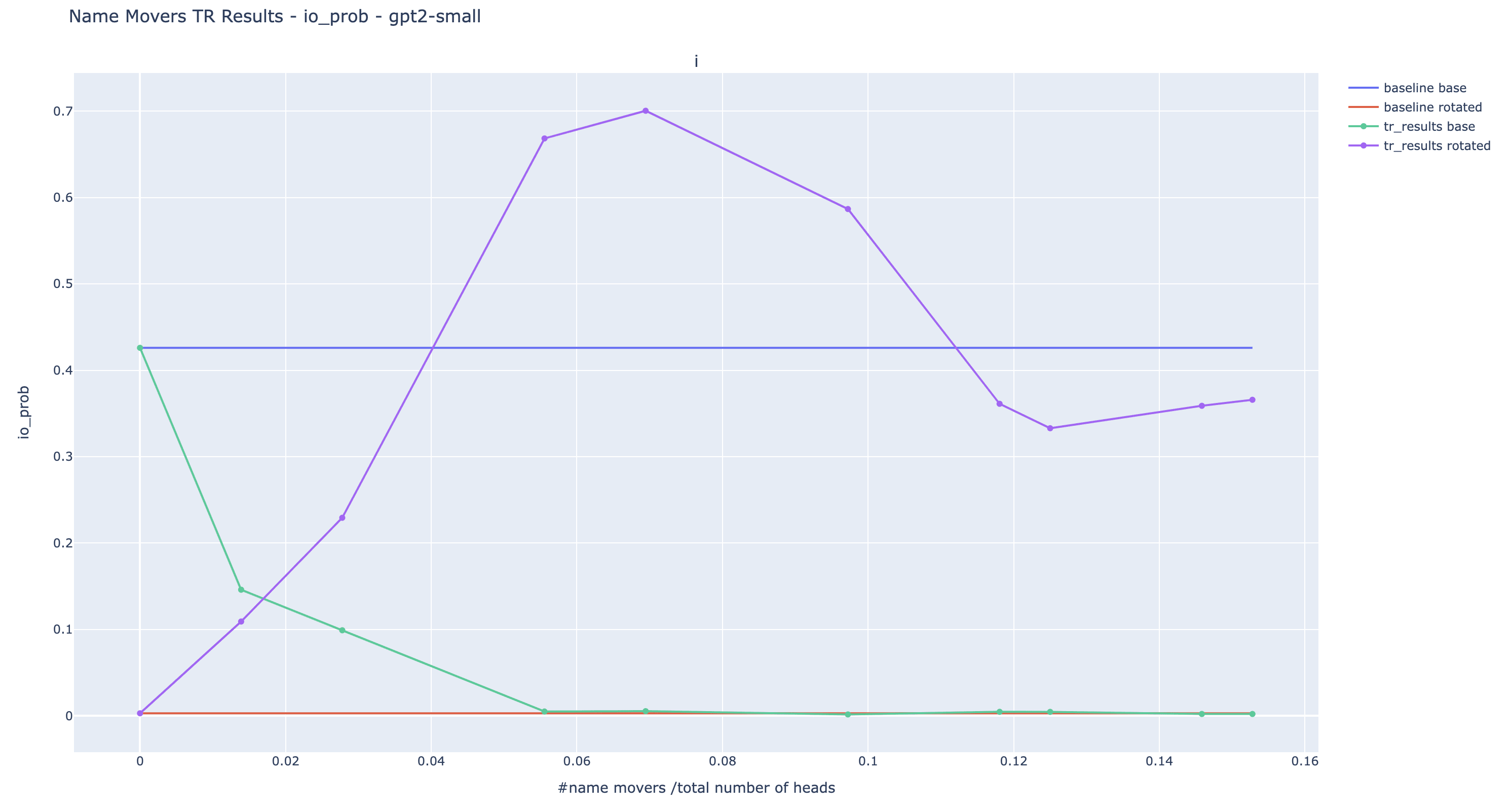
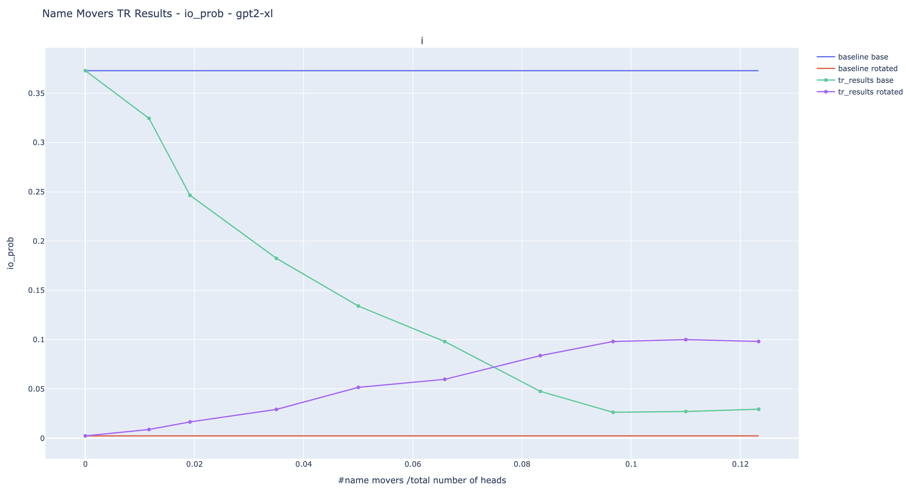
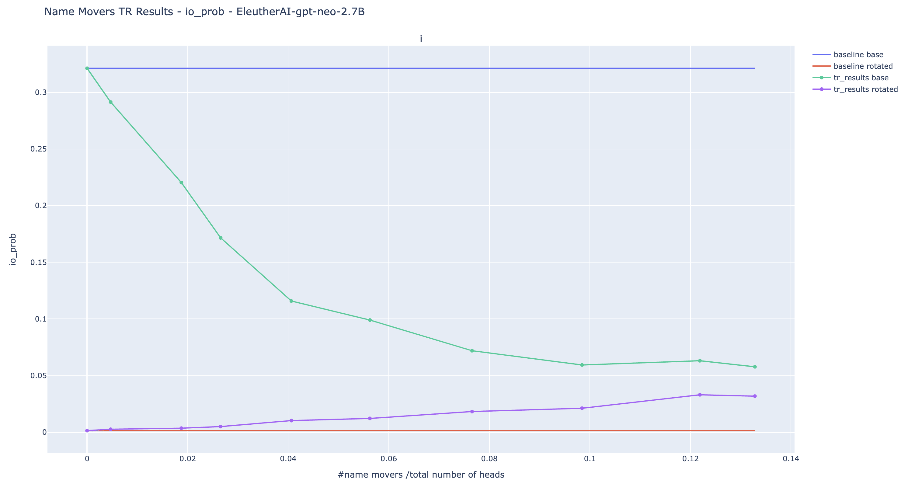
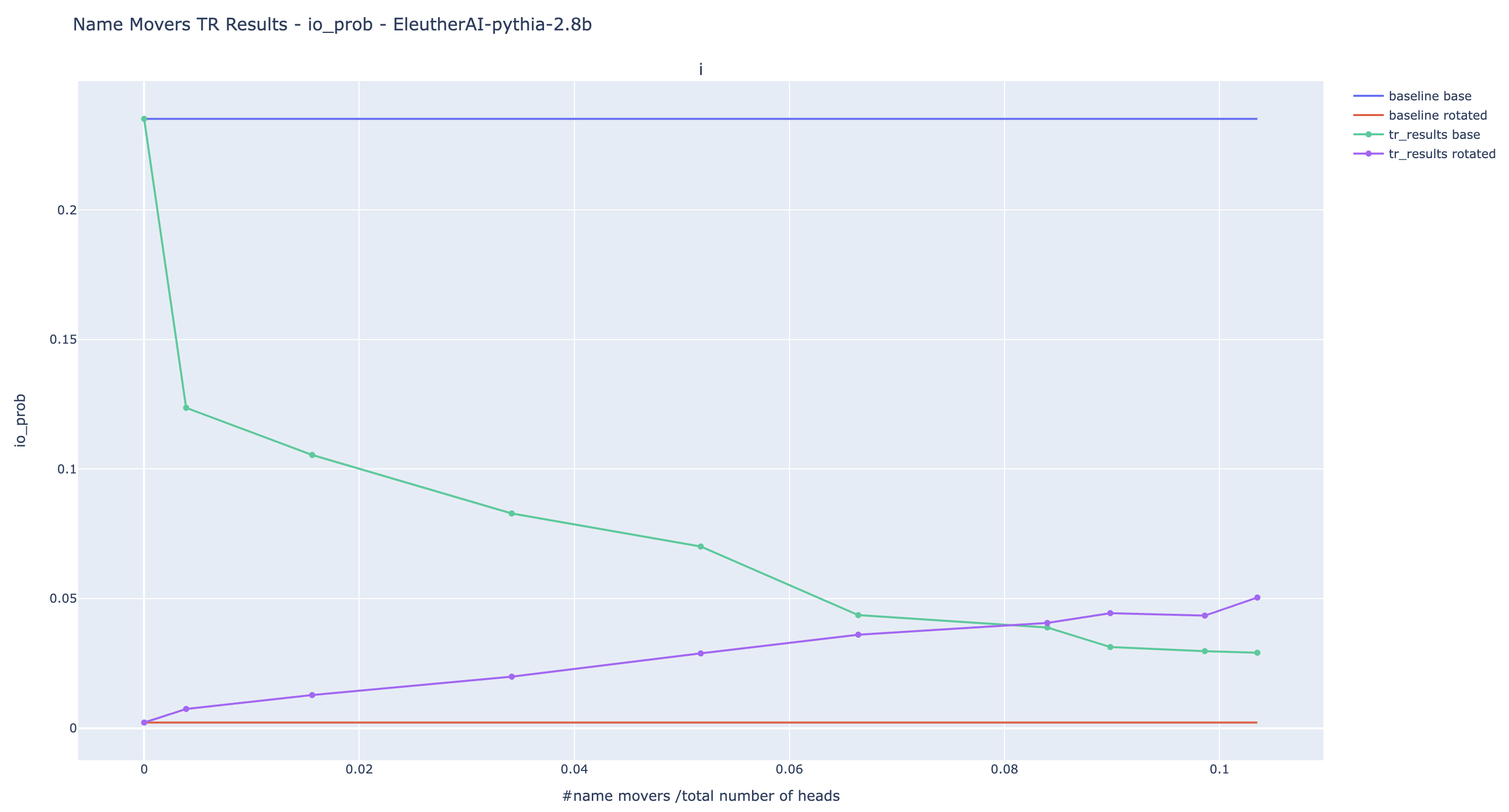
The trend observed is the one we expected: the more name movers are patched, the lower the original IO probability, and the higher the rotated IO probability. Nonetheless, despite patching more than 10% of the heads, we are unable to reach probabilities of the same order as the original IO probability in large models. It is a limitation of the current experiments: we cannot totally rewrite the output with targeted causal intervention.
Note about negative heads: The bump visible in the plot of GPT2-small is due to Negative Name Movers. Adding Negative Name Movers causes the rotated IO probability to decrease suddenly. They are likely to be also present in the other models but their effect is compensated by positive name movers.
I made the choice to design criteria for finding extended name movers that treat equally positive and negative heads -- heads that systematically write again the direction of the most probable answer, the IO token in this case. Negative and positive heads create an equilibrium and there is no obvious reason to separate them if they’re doing the same role but with opposing effects. If we are good enough to understand the underlying mechanism, we should then be able to steer the whole equilibrium in the direction we want.
I expect that if we filter for negative heads, we can make large models output with high probability by patching only a few heads. But I am not interested in these targeted rewrites as they push the model to an unnatural equilibrium.
Targetted rewrites of senders components
In semantic maps, we identified heads that encoded for the position, the S token, and the S gender. We hypothesized that they might play an analogous role as the S-Inhibition heads in IOI. They would be sending information related to S like its position, its value, or its gender. This would be responsible for name movers' attention specific to the IO token and inhibiting attention to S. The goal of this rewriting is to flip the token outputted by the model by making extended name movers copy the S token instead of IO.
Here, we’ll test this hypothesis by defining sender components and performing targeted rewrites on them.
A component C (attention head or MLP block) is a sender of the feature iff
- C is in the 90th percentile in importance among the other components at the END position. Importance is measured by average KL divergence between the original and patched model output where has been randomly resampled in .
- Its adjusted Rand index between the Louvain communities of its swap graph and the feature is in the th percentile among components.
Compared to the definition of extended name movers, we added the constraint about importance. This is to ensure that we are not picking un we are not picking up on heads that are tracking features but only weakly used in this context.
Another crucial difference is that we allow MLP blocks to be senders. As observed in the semantic maps, they have Rand indices that sometimes correlate with S features, it makes sense to include them.
We gathered the sender of the ABB/BAB template type, S token, and S gender. Then, we flipped the information contained in the sender components so that instead of matching the characteristics of the S1 position and the S token, they instead match the characteristics of IO.
- For the position senders, we swapped their input such that they see a sentence with an opposed template type. The exact sentence was randomly selected among all the sentences with this type.
- For the S token senders, we swapped their input for a sentence where the S token played the role of the indirect object.
- For the S gender, we swapped their input for a sentence where the S gender is the same as the IO gender from the original sentence.
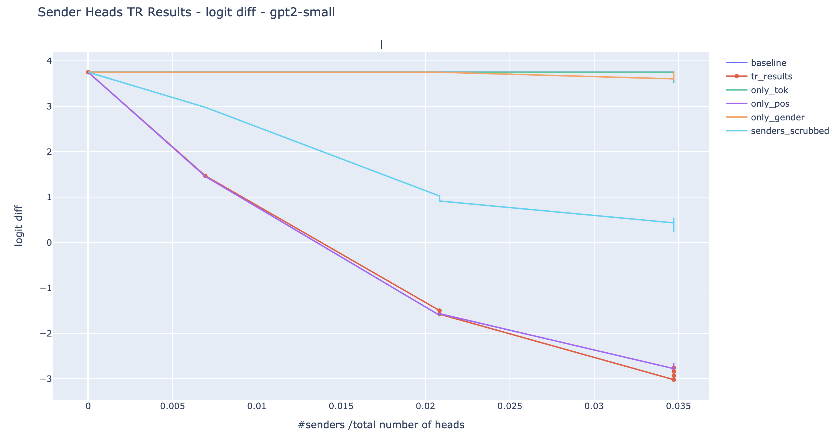
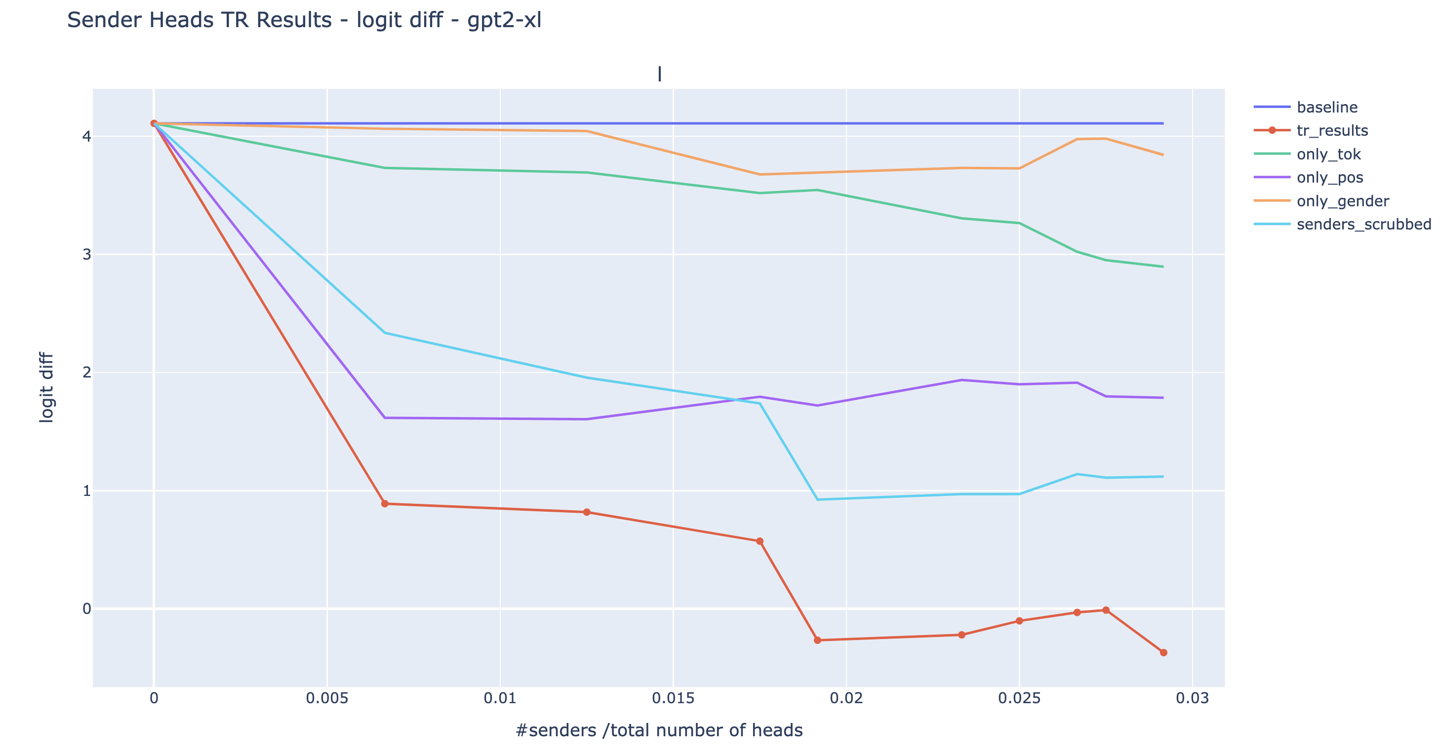
Here are the results for various choices of . In addition to doing all three swaps at the same time (red line), we also conducted them individually to see which type of sender have the most impact (orange, purple, and green line). We included a baseline where instead of swapping the input to the senders such that their output matches the characteristics of IO, we simply ablate them by arbitrarily resampling their input (light blue).
In this case, the logit diff is the natural metric to quantify the success of the operation as it directly measures how much the model is outputting S more than IO. You can still find the results with more metrics in the drive folder.
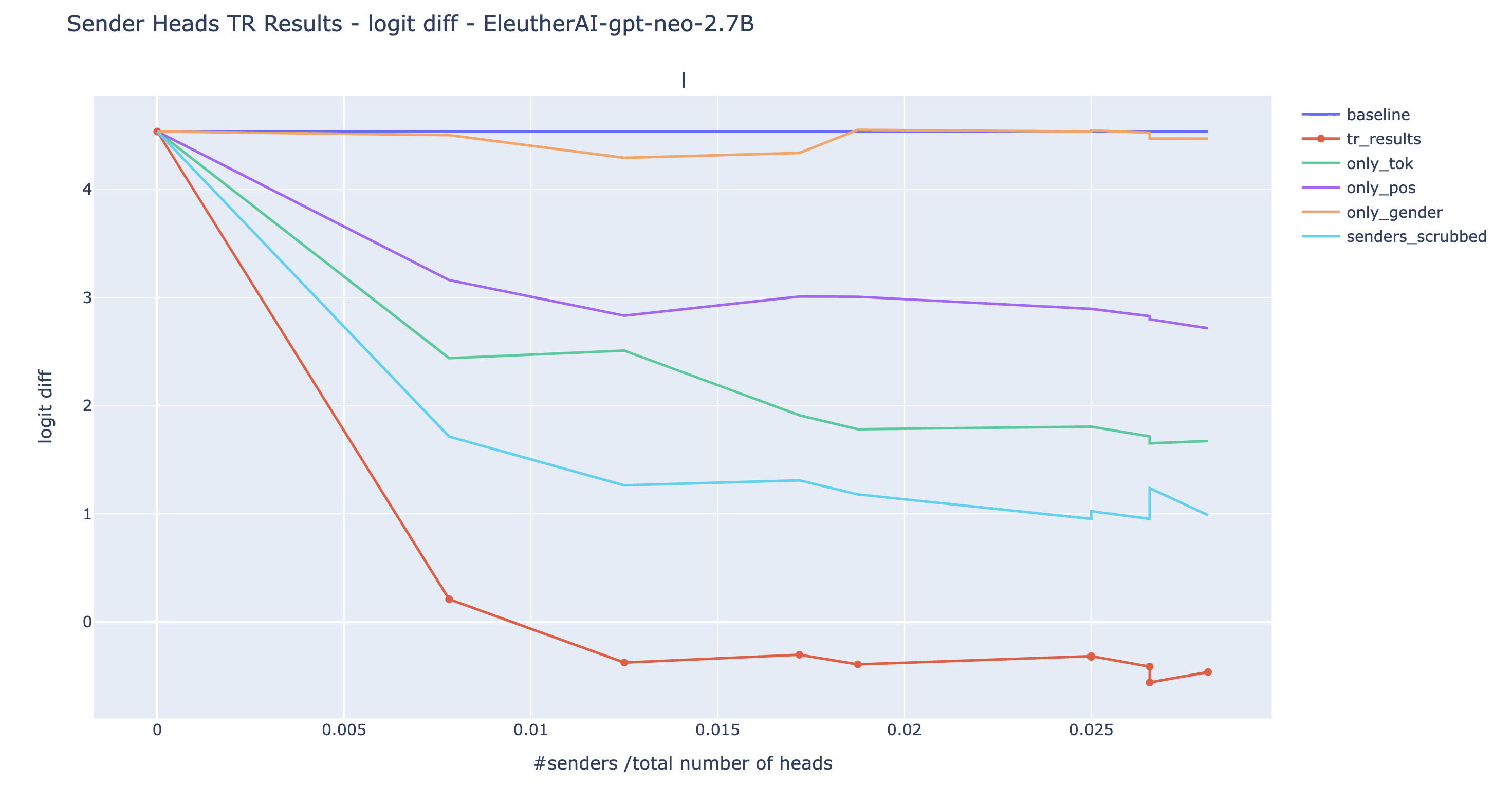
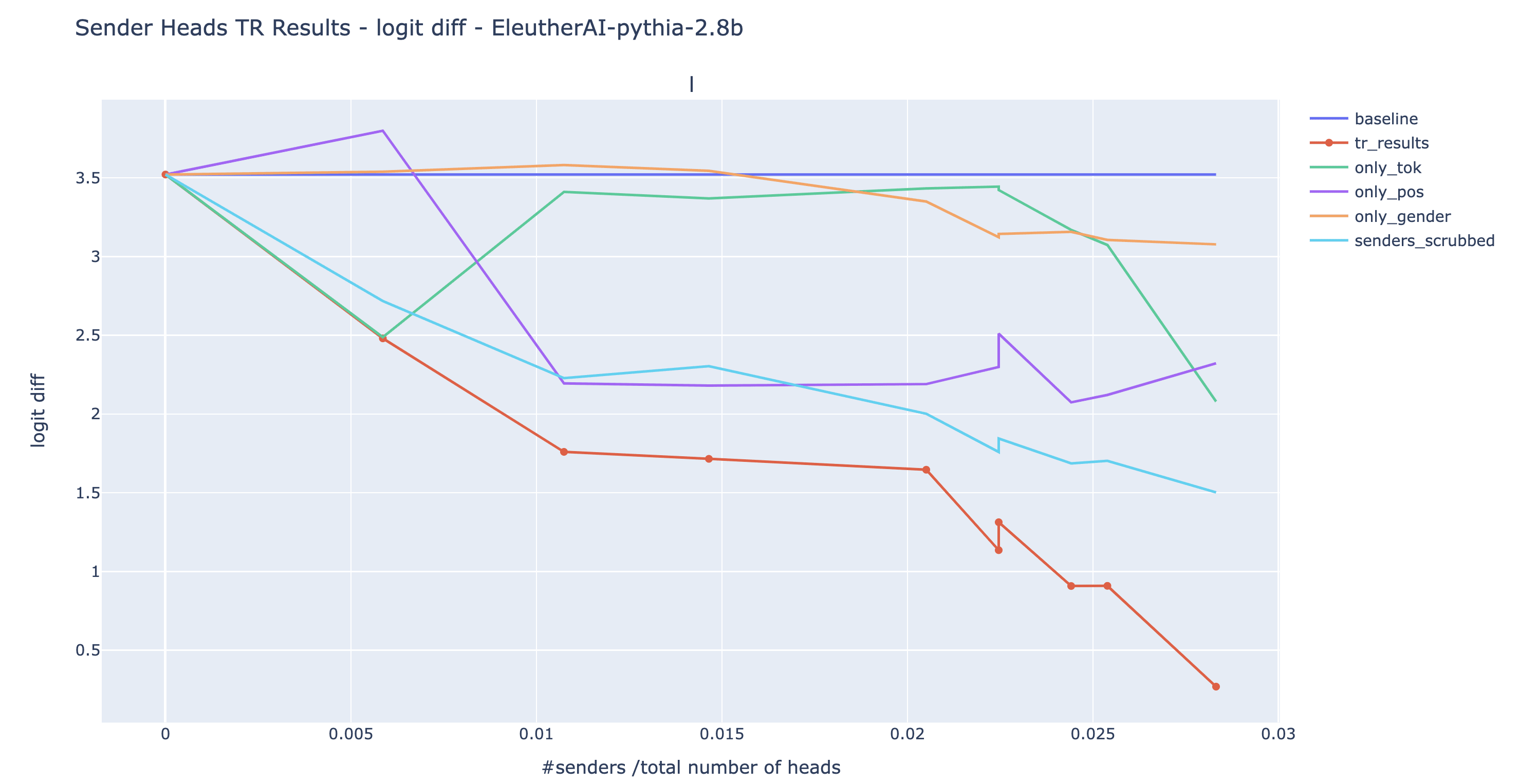
Observations/comments:
- For GPT2-small, the targeted rewrite is a near-total success. The model is outputting S with as roughly as much confidence as it would output IO under normal circumstances (logit diff=-2.9 after rewrite, vs +3.8 normally).
- The light blue line is always above the red line. This means that ablating the senders is always less effective than swapping their input according to their role given by the semantic maps. This shows that the targetted rewrites results cannot be solely explained by the fact that we arbitrarily broke the mechanism: the information from the semantic maps matters.
- For three out of the four models, we can make the model output S with greater probability than IO (logit diff <0) by patching less than 3% of the heads. This is additional evidence that we're not just breaking the mechanism and making the model predict IO and S to the same level. Nonetheless, we don’t have a full reversal of the logit diff as we observe in GPT2-small.
- When we observe a negative logit diff (GPT2-XL and Neo), we also find that the extended name movers (with ) attention probability to the S1 token position exceeded the attention probability to the IO token. When the logit diff is the most negative, the attention probabilities from END to S and IO respectively change from (0.05, 0.46) to (0.23, 0.21) for GPT2-XL and from (0.04,0.40) to (0.17, 0.18) for GPT Neo 2.7B (see the drive folder for these plots). This is medium evidence that we are in fact making the model predict S more than IO by changing which token from the context it is copying.
- The position senders and the S-token senders seem to be the most important in all four models.
- Given the non-monotonic curves, it’s likely that Pythia has negative senders that limit the effect of the targeted rewrite.
Given our naive assumption that the conclusion about IOI on GPT2-small transfer to bigger model without e.g. checking that the senders compose with extended name movers, nor that extended name movers behave as in GPT2-small, it’s a surprisingly successful experiment.
There are many hypotheses about why targeted rewrites on large models don't work as well. For instance, they might be more robust to patching in general, or the feature we rewrote might fit less correctly the role the components are actually playing. Another likely hypothesis is that we only rewrite one information route used to predict IO, but larger models use additional circuits.
Limitations and future work
Takeaways
Swap graphs for exploratory interp
The high throughput of bits makes swap graphs well-suited to design and test hypotheses about the role of components in neural networks. I think that this technique can become a crucial tool for exploratory mech interp and could improve on other techniques (hypothesis-driven patching, logit lens, etc) in many cases. I’d be excited to see it applied to other problems!
Toy theoretical model of localized computation
I found it useful for pedagogical purposes and to quickly come up with counter-examples to the naive interpretation of swap graphs. In general, it seems sane to link back messy experiments on neural networks to theoretical cases that distill one difficult aspect of the problem we’re trying to solve.
Swap graphs to understand large models
As shown with the causal scrubbing results, we can easily recover sets of inputs invariant by resampling from swap graphs. This is an important empirical foundation that legitimizes the technique despite the less significant modularity of the graphs. We can also use them to define groups of components that encode the same variables and perform targetted rewrites.
They could be a promising tool to discover high-level structures in TLM internals that appears across scale and models such as groups of components encoding the same intermediate variable in many different contexts. This could provide an exciting extension to the behavioral induction heads [LW · GW] introduced by Anthropic.
Throughout this work, I mostly rushed to scale up the approach and extract information as fast as possible from the swap graphs without refining the process along the way. My rationale was that if swap graphs contain enough signal, I would not need advanced network processing. The results are encouraging and it’s likely that we could obtain better results using more advanced network processing.
Nonetheless, it is limited. We cannot use it to perfectly able to arbitrarily steer the model given our knowledge from swap graphs. I think that it’s mostly due to the fact that many swap graphs in large models don't correlate well enough with any known feature. This might be the single most important limitation. To move further, one could consider smaller components to patch that are more likely to correspond to clean variables (e.g. MLP neurons or projecting component output into subspaces). Another way could be refining our interpretation of swap graphs to deal with the case where a component encodes multiple variables at the same time.
Future works
A disordered list of possible extensions.
- Using coarse-grained interpretability with semantic maps on new high-level tasks such as question answering.
- Can we find movers and sender in such a case? Can we make the definition of mover and sender more precise? A way to validate such findings could be to craft interventions such as removing the abilities of the model to answer questions while keeping the rest of its abilities.
- Optimization: Faster swap graphs using attribution patching, a first-order, gradient-based approximation of the results patching. This could enable running swap graphs on larger datasets and extracting more signals.
- Automated dataset handling
- Automatic dataset generation. Being able to zoom in on clusters by generating inputs that keep constant the feature that correlates with a cluster (as done in the study of S-inhibition heads).
- Automatic labeling of features in clusters: ask an LLM like GPT-4 what are the common features between inputs of a cluster (similar to the recent work from OpenAI).
- The ultimate goal would be an automated pipeline where clusters are automatically discovered and labeled at different levels of detail.
- More theoretical works:
- Thinking more about the interpretation of swap graphs in the presence of continuous variables and superposition.
- Interpreting swap graphs outside of the naive interpretation. Use this to make better use of the empirical data (e.g. using other techniques than community detection).
- Sketching an algorithm that solves the problem introduced in the section "Problem setting" under various hypotheses about the processor and the program.
- Make swap graphs from other types of patching like edge patching or path patching.
- In this work, I did the minimal structural work possible, i.e. only finding the importance of components as measured by resampling ablation. The goal is to eventually combine rich structural analysis with swap graphs.
- Application: In the long term, we could use swap graph-based causal scrubbing to sanitize model components. I.e. we run high-level causal scrubbing hypotheses that force them to interact in a way we understand. This could enable guarantees that unknown mechanisms will not be triggered on out-of-distribution samples.
- Extending the causal scrubbing results by using semantic maps to limit the number of partitions used.
- We could run community detection in the semantic maps and enforce a single resampling partition for each component in the semantic map communities. It’s a good test to see if many components are basically doing the same thing or if you need to take into account the peculiarities of each of them.
- What’s the role of gender heads in IOI?
Appendix: Swap graph with logit difference
To be closer to the IOI paper, we could use the logit difference as the metric to compare the output between the patched and original model. More precisely, we have:
Here is the swap graph with this metric for the Name Mover head 9.9 (using the Gaussian kernel to turn distances into graph weights).
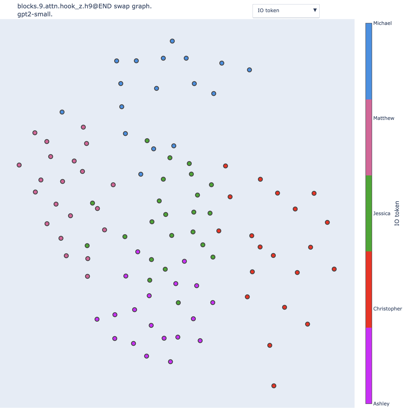
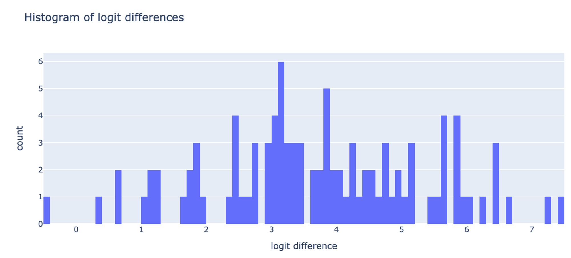
We observe a correlation between position and color, but the clusters are not as clear as when using the KL divergence. The difference is even more striking when we change the standard deviation of the Gaussian kernel, from the 25th percentile to the 5th percentile of the distribution:
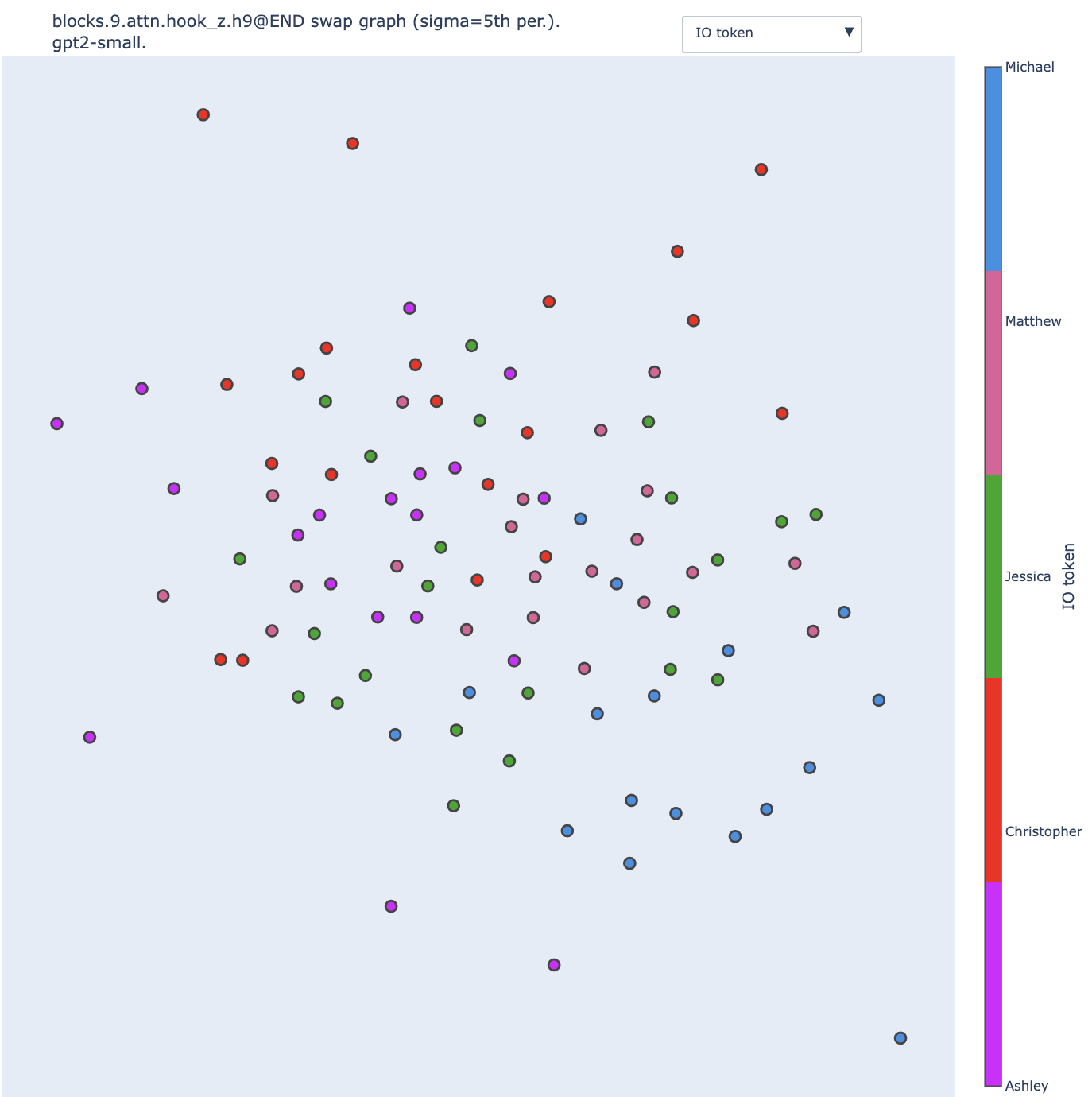
No clear cluster at all. Here is the KL divergence for comparison with the kernel with the 5th percentile.
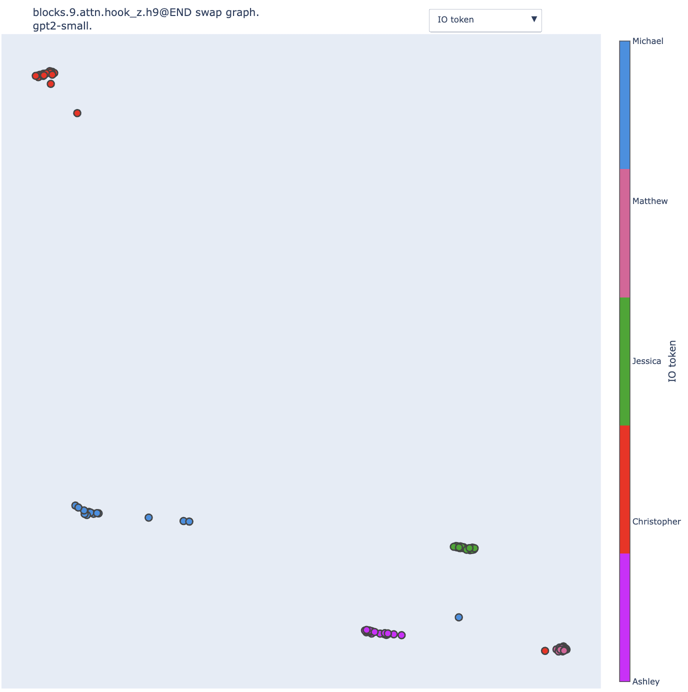
With the KL divergence, reducing the sigma makes the clusters extremely distinct. The vast majority of the input pairs that lead to swaps with KL divergence below the 5th percentile are pairs of sentences that share the same IO token (modulo some outliers involving the "bone" object, e.g. the blue dot in the middle of the red, purple and green clusters).
This is not true for logit difference: some pairs of input can be swapped without impacting much the logit difference (<5th percentile) despite involving different IO tokens.
I don't have a good understanding of why this is the case, but two factors made me decide not to use the logit diff for the rest of the study without worrying too much about this observation:
- It's a highly variable metric and we don't understand well the source of its variance (see the logit diff distribution below). That's a general red flag when we want to use it on pairs of data points and not averaged over a large sample.
- It's a one-dimensional projection of the model output. The theoretical setting suggests that this partial measure of the model output could lead to swaps causing no change "by coincidence".
Nonetheless, despite the disappointing results on Name Movers, partial investigation of heads further down suggests that the observations drawn from swap graphs on IOI hold with logit difference. For instance, here is the swap graph of the S-Inhibition head output.
- ^
Swap graphs are directed. In this context, a clique is a subset of vertices such that every two distinct vertices are connected in both ways.
- ^
Implementation is available here.
0 comments
Comments sorted by top scores.
