Uncalibrated quantum experiments act clasically

Contents

  Informal Overview
    What happens if you don't calibrate an experiment
    Possible explanation of the Born rule?
    The rest of the post
  The Experiments
    Background: Partially-silvered mirrors
    First experiment: Uncalibrated Mach-Zehnder interferometer
      Calculating the amplitude
    Second experiment:
    Third experiment:
    These uncalibrated experiments act clasically
None
12 comments

Epistemic status: solid math, uncertain applicability. Would love to hear from someone who knows more physics than I do!

Informal Overview

Here's a pretty obvious fact from probability theory:

Let A and B be two disjoint events, meaning that at most one of them can happen. For example, if you flip a coin it might land heads, or it might land tails, or it might do neither, perhaps slipping into a heating duct never to be seen again. But it definitely won't come up both heads and tails. Then:

$P(A\vee B)=P\left(A\right)+P\left(B\right)$

One of the surprising aspects of quantum mechanics is that this fact does not hold in a quantum system.

In a quantum system, an event does not directly have a probability: a real number between 0 and 1. Rather, it has an amplitude: a complex number of magnitude at most 1.

What's the meaning of this amplitude? The Born rule says that the probability that an event will be observed is the square of the magnitude of the amplitude of that event. Labeling this function $Born\left(\alpha \right)$, we have:

$Born\left(\alpha \right)={\left|\alpha \right|}^2$

The surprising fact from quantum mechanics is that when there are two ways, A and B, for something to happen, and you want to know the probability that it happens, you don't add the probabilities of A and B together. You add their amplitudes. For example, if A has amplitude $\frac{i}{2}$ and B has amplitude $-\frac{i}{2}$, then $A\vee B$ has amplitude 0. Looking at their probabilities (obtained via the Born rule), we get:

$P\left(A\right)={\left|\frac{i}{2}\right|}^2=\frac{1}{4}P\left(B\right)={|-\frac{i}{2}|}^2=\frac{1}{4}P(A\vee B)={|\frac{i}{2}-\frac{i}{2}|}^2=0$

We combined two events that could happen, to get one that can't!

However, in this post I'd like to explain how in a poorly calibrated experiment, this strange quantum behavior will vanish and be replaced with ordinary probability. First I'll give the basic explanation. Then I'll follow up with an analysis of a experiment.

(I've been using sloppy language. You wouldn't normally call events A and B disjoint, nor use the word "or". Though if you look at the setup of an actual experiment that leads to this, and describe it with ordinary language, "disjoint" and "or" are pretty fair words to use to describe the situation. I think the reason we avoid them when talking about quantum mechanics is because the behavior is so strange.)

What happens if you don't calibrate an experiment

In a quantum mechanical experiment, the phase of an amplitude can be very sensitive to the placement of the parts you use. (The phase of a complex number, when it is expressed in polar coordinates, is its angle.) For example, a photon's phase continuously changes as it travels. Every 700nm (for red light), it goes full circle. So if your experiment involves a photon traveling from one component to another, and their placement is off by 350nm, that will multiply the amplitude by -1. And if they're off by 175nm, that will multiply the amplitude by i. You might guess that quantum experiments are often very finicky and need careful calibration. You'd be right.

As a result, it seems plausible that for some experiments, if you don't calibrate the experiment properly, then the phases of the amplitudes in it will be unpredictable. And sufficiently so that it could be accurate to model each of them as an independent and uniformly random variable. In this post, I explore what happens if we make this assumption.

Taking the above example, this means that instead of $A\vee B$ having a combined amplitude of $\frac{i}{2}-\frac{i}{2}$, it would have a combined amplitude of:

$\frac{si}{2}-\frac{ti}{2}$

where $s$ and $t$ are independent and uniformly random complex variables of magnitude 1.

This is an unusual kind of model: we have a probability distribution over a quantum amplitude. But that's exactly what we should have! We're uncertain about the phases, and when you're uncertain about something you model it with a probability distribution.

However, what we care about here is the probability, rather than the combined amplitude. To find it, we should take the expected value of the Born rule applied to the amplitude:

$E\left[Born(\frac{si}{2}-\frac{ti}{2})\right]$

Remember that $s$ and $t$ are uniformly random variables of magnitude 1. We can simplify this expression:

$\begin{array}{cccc}& E\left[Born(\frac{si}{2}-\frac{ti}{2})\right]& & \\ =& E\left[Born(\frac{s}{2}-\frac{t}{2})\right]& & \text{-- by symmetry}\\ =& E\left[Born(\frac{s}{2}-\frac{1}{2})\right]& & \text{-- by further symmetry}\\ =& E\left[{|\frac{s}{2}-\frac{1}{2}|}^2\right]& & \text{-- by the Born rule}\end{array}$

This is the average squared distance from the origin to a random point on a circle of radius $\frac{1}{2}$ centered at $-\frac{1}{2}$. You can solve this with an integral, and you get $\frac{1}{2}$.

Which suggests that the quantum-mechanical behavior has vanished! We now have this, which looks just like ordinary probability:

$\begin{array}{cccc}P\left(A\right)=\frac{1}{4}& & & \text{-- the random phase has no effect}\\ P\left(B\right)=\frac{1}{4}& & & \text{-- the random phase has no effect}\\ P(A\vee B)=\frac{1}{2}& & & \text{-- by above reasoning}\end{array}$

And indeed, if instead of starting with amplitudes $\frac{i}{2}$ and $-\frac{i}{2}$, we start with an arbitrary $\alpha$ and $\beta$, you can do the same math and get:

$P\left(A\right)={\left|\alpha \right|}^{2}P\left(B\right)={\left|\beta \right|}^{2}P(A\vee B)=E\left[{|s\alpha +t\beta |}^2\right]=|\alpha {|}^2+|\beta {|}^2$

That is, the probabilities of disjoint events add! We started with the rules of quantum mechanics, and obtained a rule from ordinary probability theory.

Possible explanation of the Born rule?

This feels to me like it's close to an explanation of the Born rule. The explanation would go like this:

In our big, messy, classical world we're never certain of the phase of any amplitude. And in the small, precise world of carefully crafted quantum experiments, we pin down the phases precisely. The purpose of the Born rule is to describe the boundary between these two models of the world. And the Born rule turns a deterministic quantum model (which only has amplitudes, not probabilities), into a probabilistic classical model (which only has probabilities, not amplitudes). To justify this leap, we should show that (i) there is legitimate uncertainty that cannot be eliminated by a better model, and (ii) that the laws of probability theory hold in our proposed probabilistic model. For (i), we are legitimately uncertain about the phases of the amplitudes, and there is no feasible way to fix this. For (ii), I have given an argument that disjoint probabilities add under the Born rule, which is the most important of the laws of probability theory.

The trouble with this explanation is that it's only appropriate to add amplitudes together in particular situations, and phases are only random in particular situations, and it's not clear whether these sets of situations overlap much. In the rest of this post, I precisely describe a situation in which they do overlap. Hopefully this can give us a clearer picture of how realistic this explanation is.

The rest of the post

In particular, I work through a particular experiment (similar to a Mach-Zehnder interferometer), showing in more detail how you can get into the above situation of adding amplitudes that have random phases. To give an outline:

1. I describe three experiments with partially-silvered mirrors. Importantly, they are uncalibrated, i.e. their components are not precisely placed. I give a precise definition of what counts as "uncalibrated".
2. I show that using the Born rule $|\alpha {|}^2$, the outcome of the experiment can be predicted with classical probability, but using the (incorrect, but plausible) alternative rule $\left|\alpha \right|$, it cannot be.

The Experiments

The three experiments use a single-photon light source, partially-silvered mirrors, and a photon detector. The second and third experiments are minor variations on the first. In every experiment, what the experimenter cares about is whether the detector beeps.

Background: Partially-silvered mirrors

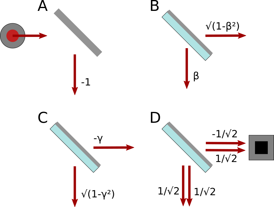
Here are diagrams for how a photon interacts with a partially silvered mirror. It can either go straight through or reflect off, and the amplitude of each possibility depends on how silvered the mirror is (an unsilvered mirror would just be glass), and how it is oriented:

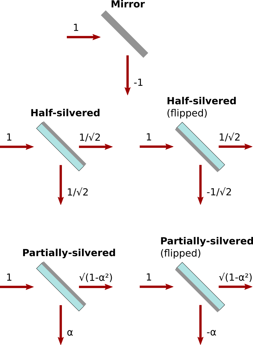
(The amplitude $\alpha$ is an unspecified real number between 0 and 1. If it's $\frac{1}{\sqrt{2}}$, then the mirror is half-silvered. If $\alpha$ is smaller it's less than half-silvered, and if $\alpha$ is bigger it's more than half-silvered.)

Let's work through an example of how to use these diagrams to predict the outcome of an experiment made up of some mirrors, a single-photon light source, and a photon detector. To determine the probability that the detector beeps, you should:

1. Consider all paths from the light source to the detector.
2. Determine the amplitude of each path, by multiplying the amplitudes of each of its steps.
3. To determine the amplitude of the outcome in which the detector beeps, add together the amplitudes of each path that leads to the detector.
4. To determine the probability of the outcome, use the Born rule: take the absolute value of the amplitude and square it.

Those are the rules. Let's apply them to a simple example experiment:

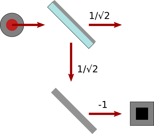
Applying the rules:

1. There's only one path that leads to the detector. It goes right, down, right.
2. We multiply the amplitudes we see along the path ($\frac{1}{\sqrt{2}}$ and $-1$) to get $-\frac{1}{\sqrt{2}}$.
3. If there were other paths, we'd add their contributions too. But there's only one so our total amplitude is $\frac{-1}{\sqrt{2}}$.
4. By the Born rule, the probability of the detector beeping is ${\left|\frac{-1}{\sqrt{2}}\right|}^2=\frac{1}{2}$.

That's all there is to it.

First experiment: Uncalibrated Mach-Zehnder interferometer

Here's the setup of the first experiment:

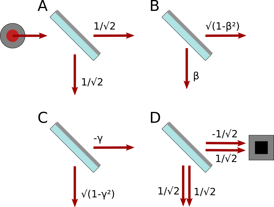
Note that B and C are partially silvered, but need not be exactly half-silvered. I call their amplitude of reflection $\beta$ and $-\gamma$ respectively. There's one tricky thing going on here, on the path from D to the detector. This amplitude is either $\frac{-1}{\sqrt{2}}$ or $\frac{1}{\sqrt{2}}$, depending on whether the incoming photon came from B or C, respectively. (This follows from the diagrams I gave for the mirrors. I'm not just making it up!)

(If you know what a Mach-Zehnder interferometer is, this setup is the same except that B and C are only partially-silvered, allowing the photon to sometimes escape into the air.)

There's one other crucial feature for this setup, which is the point of this post. I gave an intuitive argument in the introduction that an experiment like this is extremely sensitive to the placement of its parts and must be carefully calibrated. I'm going to assume that this setup was not carefully calibrated, its parts are not fastened down, and as a result the phase of a photon taking any path is, for all practical purposes, uniformly random. More precisely:

Strong Uncalibration Assumption: The phase change of a photon traveling through the apparatus can be accurately modeled as uniformly random. Furthermore, the phase change of a photon is independent from one run of the experiment to the next, and the phase change along the top path is independent of the phase change along the bottom path.

Honestly, I'm not sure how realistic this assumption is; I'm relying on intuition here. But if it does hold, it gives a very satisfying account of how quantum mechanics degenerates into ordinary probability when things are uncalibrated. I'd love to hear from a physicist on the matter.

Calculating the amplitude

Let's see how that works. First, what is the amplitude that the detector beeps?

There are two paths to consider: A-B-D-detector, and A-C-D-detector. Their contributions are:

$\begin{array}{cccc}\text{Top path (A-B-D):}& \frac{1}{\sqrt{2}}\ast \beta \ast \frac{-1}{\sqrt{2}}& =& \frac{-\beta }{2}\\ \text{Bottom path (A-C-D):}& \frac{1}{\sqrt{2}}\ast -\gamma \ast \frac{1}{\sqrt{2}}& =& \frac{-\gamma }{2}\\ \text{Total:}& \frac{-\beta }{2}-\frac{\gamma }{2}& & \end{array}$

However, that is only true if the experiment is perfectly calibrated. We are assuming instead that it is uncalibrated, and that the phases of the paths can be modeled as uniformly random.

I'll be talking a lot about uniformly random phases, so I'll introduce some notation for it. Define $⨀$ to be the probability distribution of a complex number chosen uniformly at random the unit circle. For example:

• $\frac{s}{2}\text{where}s\sim ⨀$ is a uniformly random amplitude with magnitude $\frac{1}{2}$.
• $\frac{s}{2}-\frac{i}{4}\text{where}s\sim ⨀$ is an amplitude chosen uniformly at random from a circle with radius $\frac{1}{2}$ centered at $\frac{i}{4}$.

Using this notation, we can correct our calculation of the total amplitude by accounting for the random phases caused by the uncalibrated setup:

$\text{AMPLITUDE\_1}=\frac{-s\beta }{2}-\frac{t\gamma }{2}\text{where}s,t\sim ⨀$

(I'm calling this AMPLITUDE_1, as it's the result of the first experiment.)

Because the negative signs make no difference when multiplied by a uniformly random phase, this becomes:

$\text{AMPLITUDE\_1}=\frac{s\beta }{2}+\frac{t\gamma }{2}\text{where}s,t\sim ⨀$

Second experiment:

The second experiment is like the first, but with half-silvered mirror A removed:

With this setup, there is only one path to consider, A-B-D-detector. The amplitude of this path (removing an unnecessary negative sign) is:

$\text{AMPLITUDE\_2}=\frac{s\beta }{\sqrt{2}}\text{where}s\sim ⨀$

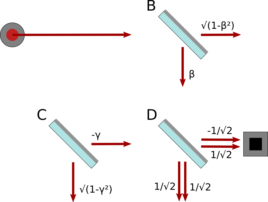
Third experiment:

The third experiment is like the first, but with the half-silvered mirror at A replaced with a full mirror:

Now there is only the path A-C-D-detector, with amplitude:

$\text{AMPLITUDE\_3}=\frac{s\gamma }{\sqrt{2}}\text{where}s\sim ⨀$

These uncalibrated experiments act clasically

Using the Born rule, we can determine the probability of the photon being detected in each of the three experiments. Since in each case we have a probability distribution over a quantum amplitude, we will take the expected value of the Born probability:

$\begin{array}{cccc}E\left[Born\left(\text{AMPLITUDE\_1}\right)\right]& =E\left[{|\frac{s\beta }{2}+\frac{t\gamma }{2}|}^2\right]\text{where}s,t\sim ⨀& & =\left(\right|\beta {|}^2+\left|\gamma {|}^2\right)/4\\ E\left[Born\left(\text{AMPLITUDE\_2}\right)\right]& =E\left[{\left|\frac{s\beta }{\sqrt{2}}\right|}^2\right]\text{where}s\sim ⨀& & =|\beta {|}^2/2\\ E\left[Born\left(\text{AMPLITUDE\_3}\right)\right]& =E\left[{\left|\frac{s\gamma }{\sqrt{2}}\right|}^2\right]\text{where}s\sim ⨀& & =|\gamma {|}^2/2\end{array}$

(I omit the proofs, but have evaluated these integrals by hand and checked the results with Wolfram Alpha.)

This is classical behavior! Naive classical reasoning would proceed as follows:

• In the first experiment, the photon hits the half-silvered mirror at A, and either goes straight or reflects down with equal probability.
• If it goes straight through A, then it has the same chance of hitting the detector as the photon in the second experiment.
• If it reflects off of A, then it has the same chance of hitting the detector as the photon in the third experiment.
• Thus the probability of the detector going off in the first experiment is the average of the probability that it goes off in the second and the probability that it goes off in the third.

Which matches the conclusion: $\left(\right|\beta {|}^2+\left|\gamma {|}^2\right)/4$ is the average of $|\beta {|}^2/2$ and $|\gamma {|}^2/2$.

We can also work backwards, and take it as a given that this uncalibrated experiment should act classically. Doing so yields an equation that must constrain the Born rule:

$\begin{array}{cccc}& 2E\left[Born(\frac{s\beta }{2}+\frac{t\gamma }{2})\right]& & \text{where}s,t\sim ⨀\\ =& E\left[Born\left(\frac{s\beta }{\sqrt{2}}\right)\right]+E\left[Born\left(\frac{t\gamma }{\sqrt{2}}\right)\right]& & \text{where}s,t\sim ⨀\end{array}$

One obvious alternative to the Born rule is to simply take the magnitude of the amplitude, $\left|\alpha \right|$ (why would you square it?). However, doing so violates the above equation, so it would not produce classical probability. I'm not sure if this equation has a unique solution, but it is at least quite restrictive.

12 comments

Comments sorted by top scores.

E[Born(sa + tb)] = Born(sa) + Born(tb)    when s, t ~ ⨀