SAEs you can See: Applying Sparse Autoencoders to Clustering

post by Robert_AIZI · 2024-10-28T14:48:16.744Z · LW · GW · 0 comments

Contents

  TL;DR
  Introduction
  Methods
    Datasets
    Data Embedding via Anchors
    SAE Architecture
    SAE Loss Function
    SAE Training
    Measuring Results: Cluster Entropy
  Experiments and Results
    Baseline Experiments
    Scale Sensitivity Experiment
    Data Scarcity Experiment
    Identifying Number of Features Experiment
    Visualizing Features, Encoders, and Decoders
    Improving the Random Blobs result with "Adjoint Classification"
  Takeaways for Sparse Autoencoder Research
  Limitations and Future Work
  Code
  Acknowledgements
None
No comments

TL;DR

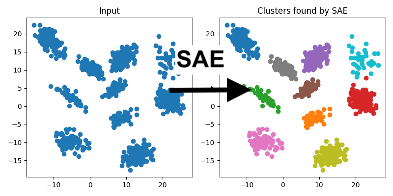
• We train sparse autoencoders (SAEs) on artificial datasets of 2D points, which are arranged to fall into pre-defined, visually-recognizable clusters. We find that the resulting SAE features are interpretable as a clustering algorithm via the natural rule "a point is in cluster N if feature N activates on it".
• We primarily work with top-k SAEs (k=1) (as in Gao et al.), with a few modifications:
  • Instead of reconstructing the original $(x,y)$ points, we embed each point into a 100-dimensional space, based off its distance to 100 fixed "anchor" points. The embedding of a point $p$ for an anchor point $a$ is roughly $\exp (-d(p,a{)}^2)$. This embedded point is both the input and target of the SAE. This embedding allows our method to identify features which are non-linear in $(x,y)$.
  • We use a variant of ghost gradients to push dead features in the correct direction. This greatly improves the reliability of the training.
• We achieve great data-efficiency (as low as 50 training data) by training for thousands of epochs.
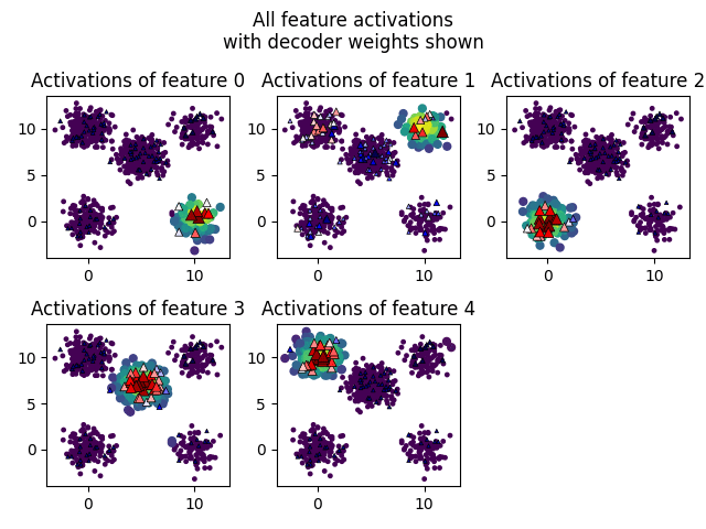
• This approach allows one to "see" SAE features, including their coefficients, in a pleasant way:

Introduction

Using Sparse Autoencoders for dictionary learning is fundamentally an unsupervised learning task: given some data, find the important things in it. If SAEs are good at that, they should be able to solve other unsupervised learning problems. Here, I try to use SAEs on a classic unsupervised learning problem: clustering 2D data. The hope is that SAEs can learn features corresponding to "in cluster 1, in cluster 2, etc". 

We investigate this on artificial data, and find that SAEs semi-reliably find the correct classification, with interpretable activations and decoder weights. 

Methods

Datasets

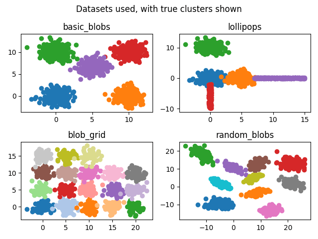
We made four synthetic datasets, consisting of separate, visually-identifiable clusters. 

1. "Basic Blobs" - 5 clusters. Points $(x,y)$ are drawn from normal distributions$X\sim N(x_{center},1),Y\sim N(y_{center},1)$ where $(x_{center},y_{center})$ is the cluster center. The 5 clusters have centers $(0,0),(10,0),(0,10),(10,10),(7,5)$, forming a square pattern with one cluster in the center.
2. "Blob Grid" - 18 clusters. As with Basic Blobs, but the centers are of the form $(5i,5j)$ for $0\le i,j\le 5$, $i+5j<18$, forming a grid pattern.
3. "Random Blobs" - 10 clusters. Points are sampled from a multivariate normal distribution, roughly forming ovals with random centers and eccentricities. The centers of the normal distributions are resampled if they are not sufficiently far apart.

4. "Lollipops" - 5 clusters. 3 clusters as in "Basic Blobs", but with centers at $(0,0)$, $(5,0)$, and $(0,10)$, plus 2 additional clusters that form thin rectangles as "stems" of the lollipops. The first stem comes down off the $(0,0)$ blob, and the second stem comes off the $(5,0)$ to the right.

   

We use classes of varying sizes: each class is randomly assigned a relative frequency from {1,2,3,4}.

Data Embedding via Anchors

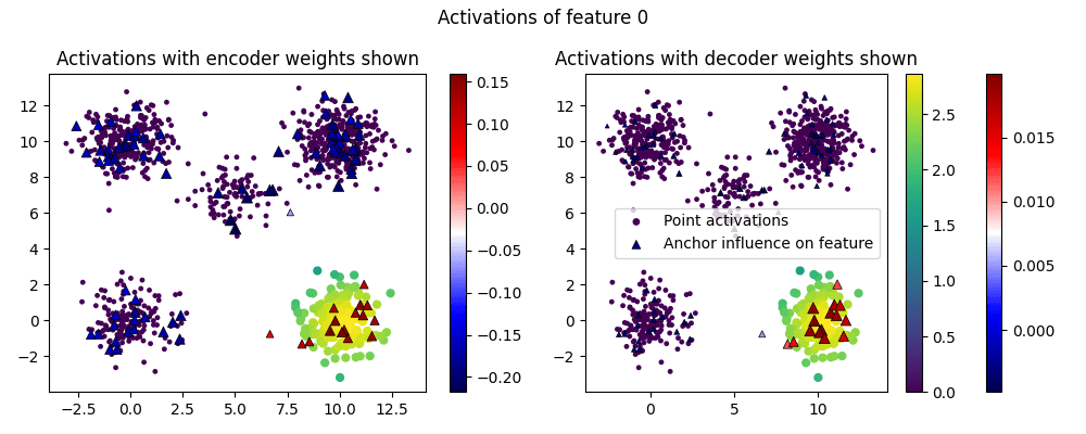
Applying a sparse autoencoder to the point cloud's $(x,y)$ points directly is extremely limited - you can at most read off a linear direction, leading to features like this one:

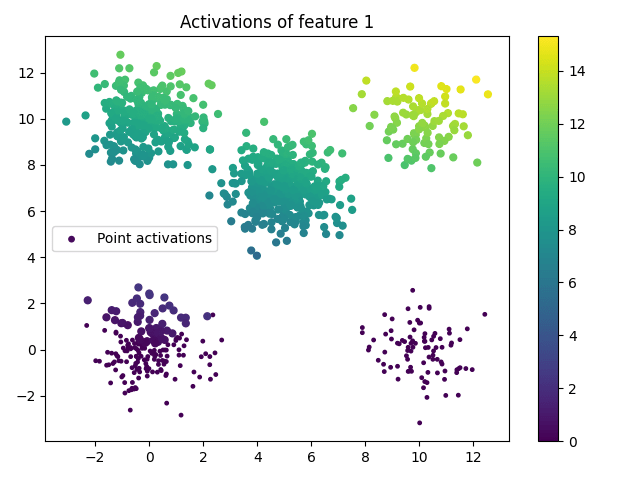
Such linear features are insufficient for the purpose of classifying. We will instead embed each $(x,y)$ point in a high-dimensional space, with the goal that clusters are linearly separable and form the natural features of the dataset, which the SAE can find.

To do this, we choose a set $A=\{a_i{\}}_{i=1}^{n_{anchors}}$ of "anchors", drawn from the same data distribution as the dataset we're training on (on real data, this would correspond to setting aside a fraction of the data as anchors). Points are encoded into $R^{n_{anchors}}$, with the $i$th encoding dimension being a function of the distance to the $i$th anchor, given by:

$embed(p{)}_i=\exp (-\frac{1}{2var(a_1,...,a_n)}\frac{1}{{\sigma }^2}\cdot d(a_i,p{)}^2)$

where $p$ is a point in our dataset, $a_i$ represents the $i$th anchor, $d$ is the usual euclidean distance, $var(a_1,...,a_n)$ is the variance of the set of anchors, and and $\sigma$ is a hyperparameter controlling the neighborhood of influence of each point relative to the overall dataset. The embeddings from a single anchor look like this:

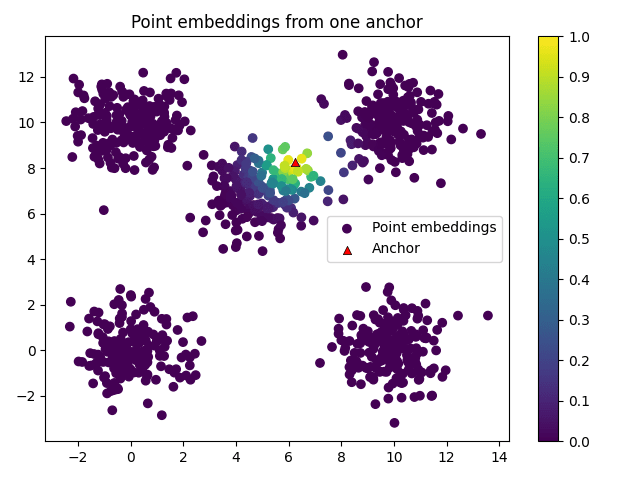
Because the embedding function is based on distances and normalized with variance, it is invariant under uniform scaling and isometries (rotations, reflections, etc).

SAE Architecture

We use an SAE architecture based on the one in Towards Monosemanticity, but with ReLU followed by top-1 as our activation function. The SAE computation is:

$\begin{array}{ccc}f& =& act\left(W_e\right(x-b_d)+b_e)\\ \tilde{x}& =& W_{d}f+b_d\end{array}$

where $x\in R^{n_{anchors}}$ is an embedded point from the point cloud, $W_e\in R^{n_{features}\times n_{anchors}}$, $W_d\in R^{n_{anchors}\times n_{features}}$, $b_d\in R^{n_{anchors}}$, $b_e\in R^{n_{features}}$ are the weights and biases of the encoder and decoder, and $act$ is ReLU followed by top-1 activation. We normalize the columns in $W_e$ and $W_d$ at inference time.

A top-k SAE has two hyperparameters: the number of features, and $k$, the number of features active at one time. We make the number of features to be the number of ground-truth classes, and take $k=1$. 

The way we embed our point cloud also has two hyperparameters, $\sigma$ and $n_{anchors}$. We use $\sigma =\frac{2}{n_{classes}}$ and $n_{anchors}=100$, which were chosen because they anecdotally work well.

SAE Loss Function

Our main loss function is reconstruction loss:

$L_{rec}\left(x\right)=||\tilde{x}-x|{|}_2^2$

Since top-1 SAEs can easily acquire dead features, we supplement this with a version of ghost grads. Following Anthropic, we designate a feature as dead if it has not activated in a significant number of previous data, in our case 1000. To compute the ghost grads, we perform the following procedure:

1. Compute the error-weighted average residual stream over the batch: ${\overline{x}}_{err}=\frac{{\sum }_x{L}_{rec}\left(x\right)x}{{\sum }_x{L}_{rec}\left(x\right)}$, and similarly the error-weighted average error direction: ${\overline{d}}_{err}=\frac{{\sum }_x{L}_{rec}\left(x\right)(x-\tilde{x})}{{\sum }_x{L}_{rec}\left(x\right)}$.
2. For each dead feature, add a loss term based on how its encoder direction aligns with ${\overline{x}}_{err}$ and how its decoder direction aligns with ${\overline{d}}_{err}$. In particular, we compute:$L_{ghost}=\sum _{\text{dead feature}{f}_i}\left(softplus\right(-{\overline{x}}_{err}{W}_e^i)+softplus(-{\overline{d}}_{err}{W}_d^i\left)\right)$.^[1]

The overall loss of the SAE is:

$L=L_{rec}+L_{ghost}$

Our ghost loss is very direct and very crude: it pushes dead features to activate on high-error features (which are presumably an as-yet-unidentified cluster), and for their decoder directions to fix the error. Nonetheless, it is sufficient for our purposes, effectively eliminating dead features, and improving reliability of training runs, especially on harder datasets.

SAE Training

Our training methods are mostly routine: we use the AdamW optimizer with learning rate 1e-4 and otherwise default parameters.

The one notable exception is the number of epochs: since clustering often suffers from limited data availability, we restrict ourselves to $n_{train}=1000$ points in our training set^[2], trained for 500 epochs. 

Counting both the training data and anchors, this results in 1100 total samples in our point cloud. Classes can be as small as ~40 points if they have a low relative frequency (see the Datasets section). We run experiments with fewer training points (see below) and find that the model can learn the correct classification on as few as 50 training points (+100 anchors), though with reduced reliability.

Our SAEs are extremely small (the number of parameters is roughly$2\ast n_{features}\ast n_{anchors}\approx 2000$, depending on the dataset being classified), so training completes quickly, in <10 seconds on my laptop.

Measuring Results: Cluster Entropy

We measure effectiveness of our model in two ways: reconstruction loss (unlabelled), and cluster entropy (using the generating clusters as labels). Cluster entropy is computed with this method^[3]: 

1. Use the true labels to partition each cluster. Measure the entropy of each cluster individually.
2. Average the entropy across clusters, weighted by the size of the clusters.

For $N$ true classes and $N$ clusters, the entropy lies in the range $[0,\log (N\left)\right]$, where lower is better. Based on my visual inspection of clusters, entropy=0.1 is the cutoff between correct and incorrect clusterings.

Experiments and Results

Baseline Experiments

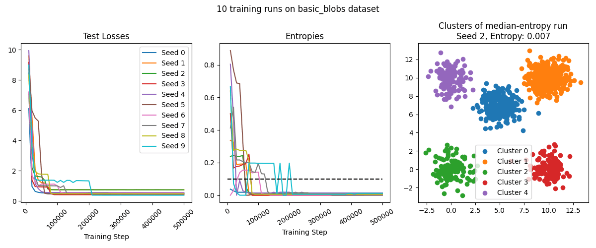
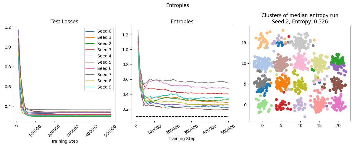
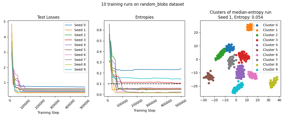
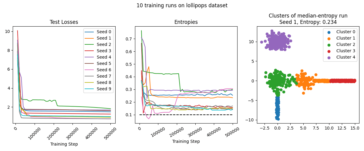
We ran the training setup described above on all four datasets. On basic_blobs and random_blobs, the SAE typically performs very well, resulting in ~perfect classification in the median case. The model is more confused on blob_grid dataset - it often identifies several clusters mostly-correctly, but struggles on several other clusters (though see the later sections for improvements on our technique that make it succeed on this dataset as well). On the lollipops dataset, the SAE has poor entropy because while it correctly finds the division of lollipops into cores and sticks, it splits them in the wrong location.

Scale Sensitivity Experiment

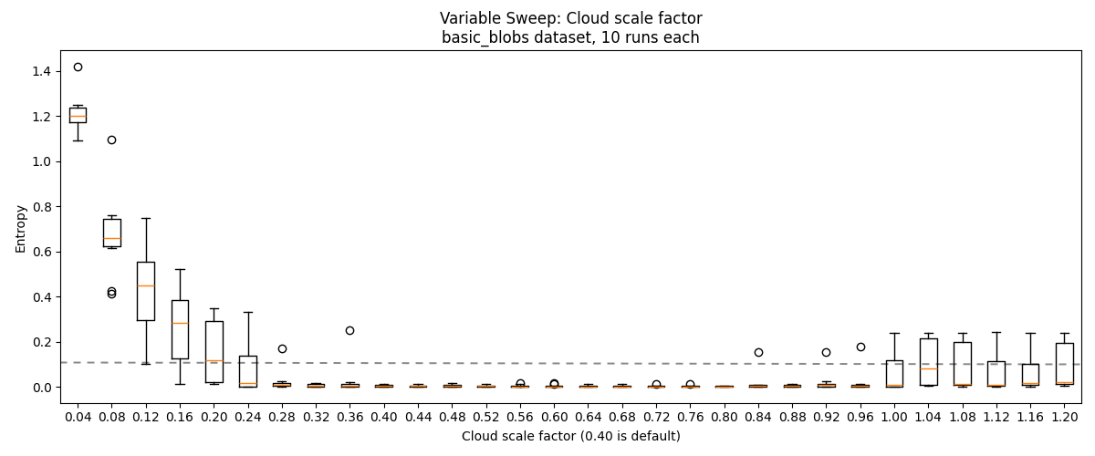
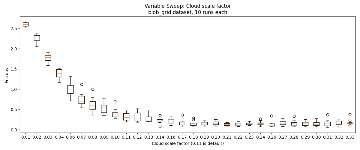
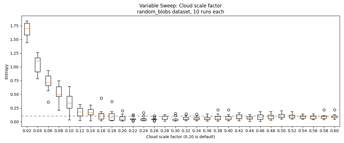
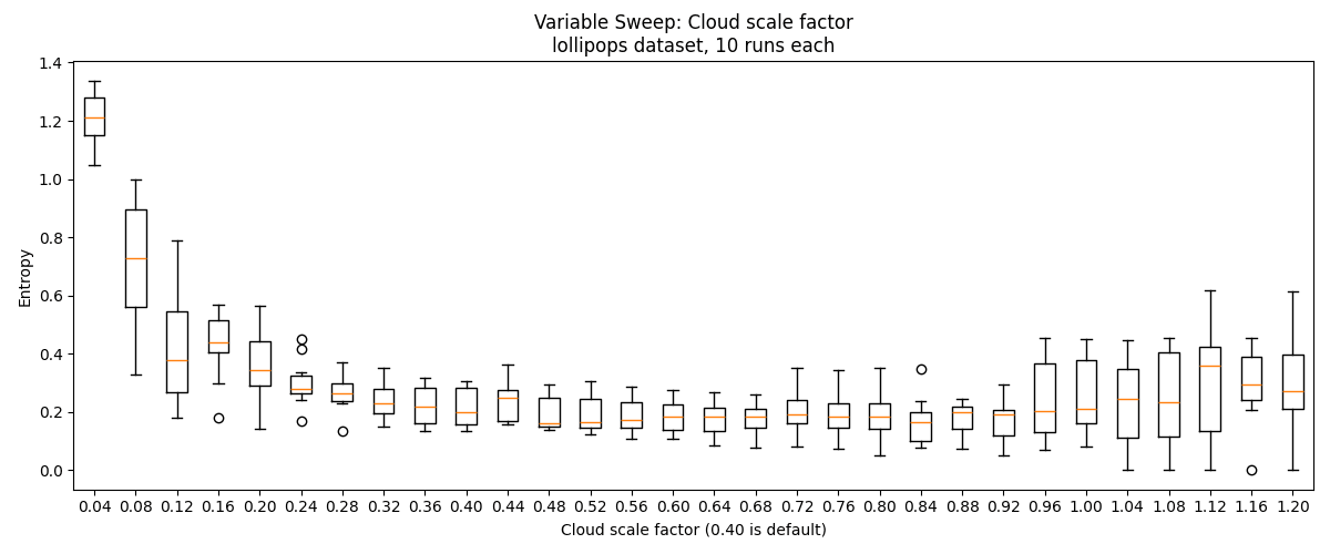
Our method relies on the hyperparameter $\sigma$, which changes the region of influence of each anchor, analogous to $ϵ$ in DBSCAN. I ran a hyperparameter sweep of this on the basic_blobs and random_blobs datasets to assess the method's sensitivity.

We find that performance drops if $\sigma$ is too large or too small. For the easier basic_blobs dataset, we get ~perfect performance for $\sigma \in [0.28,0.96]$. For the harder random_blobs and blobs_grid datasets, we get reasonably go good performance for $\sigma >0.2$, but presumably performance tapers off sufficiently large $\sigma$. On the lollipops dataset, performance is best for $\sigma \in [0.3,.9]$.

Data Scarcity Experiment

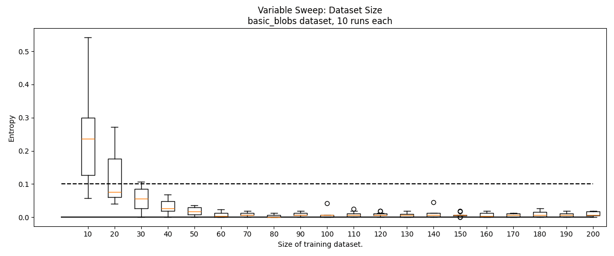
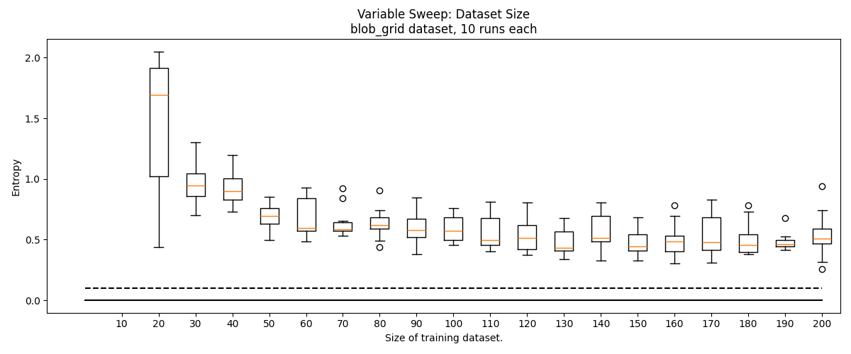
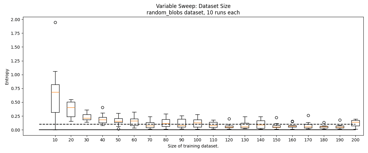
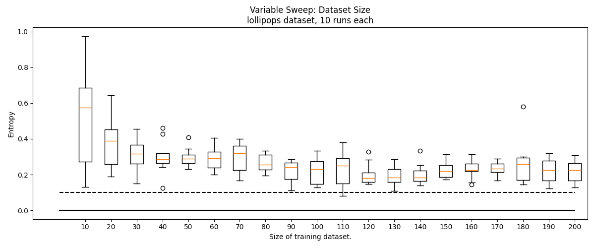
Since point cloud data is often scarce, we experimented with greatly reducing the size of our training set from the "default" $n_{train}=1000$. In this experiment, we sweep $n_{train}$ through $10,20,30,...,200$, compensating for smaller dataset size by increasing epochs to $n_{epochs}=500,000/n_{train}$. In these experiments, we keep a constant $n_{anchors}=100$.

We find that some minimum amount of data is needed for good clustering, but this threshold is surprisingly low. We typically stop seeing performance improvements around by 100 data, though for the blob_grid and lollipops datasets, this performance is poor. On the easier basic_blobs dataset, as low as 50 data can produce reliably accurate clusters (the smallest cluster in the training set will consist of ~4 points).

Identifying Number of Features Experiment

So far, we've helped our SAE by setting its hyperparameter $n_{features}=n_{classes}$. But often in clustering one does not know $n_{classes}$. Can we use the SAE to determine the correct number of features?

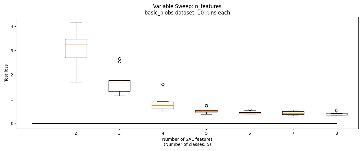
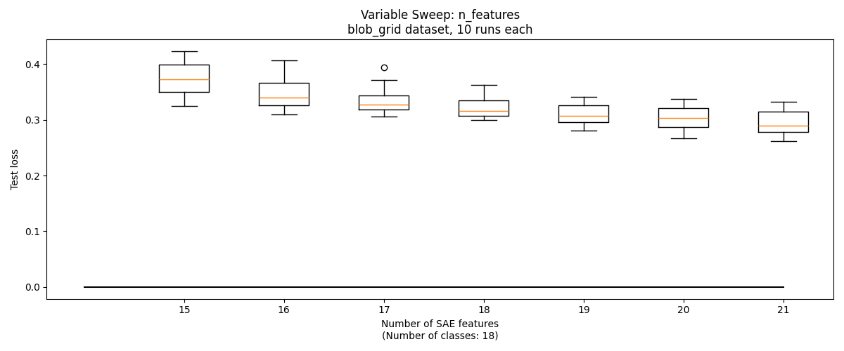
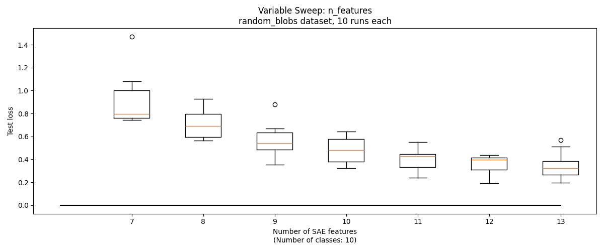
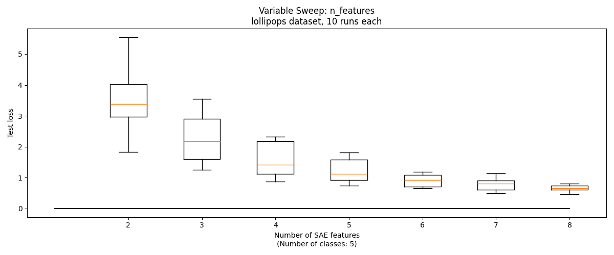
One approach is this: assume that the SAE will have high reconstruction loss if its features straddle multiple classes. Therefore, loss will be high when $n_{features}<n_{classes}$, but will be roughly similar for $n_{features}\ge n_{classes}$. We can sweep $n_{features}$, and identify the point at which adding another feature does not significantly decrease reconstruction loss, which should occur when $n_{features}=n_{classes}$.

This technique works reasonably well on basic_blobs, with with losses leveling off starting at the correct value, $n_{features}=5$. But on the other three datsets, there is not a notable change at the correct number of features.

Visualizing Features, Encoders, and Decoders

One benefit of this approach is that the SAE operates on a very visible dataset, and this lets us create diagrams to directly see parts of the SAE, namely where the features activate, the encoder weights, and the decoder weights.

Let's look at another training run on the random_blobs dataset, which produces these classifications:

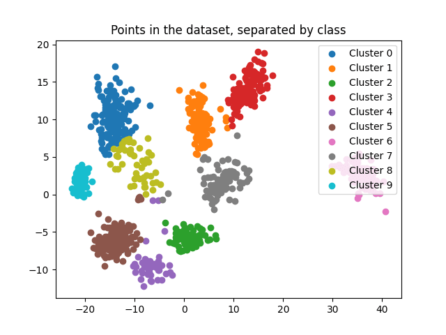
Here we can see one thing already: there is some confusion for the model, where parts of the yellow cloud are incorrectly assigned to the purple, brown, or grey cluster. These "confused points" are typically present near the fringes of a distribution, and we'll show a solution to them in the next experiment. 

What do the feature activations themselves look like? In these graphs, circular points are points in the test dataset, and their color shows whether the feature activates on them. We also draw the "anchor" points as triangles, and show the corresponding weight of the encoder/decoder in its color (redder for more positive, bluer for more negative) and size (by magnitude). 

We graph each feature twice, with the encoder weights shown on the left, and the decoder weights shown on the right:

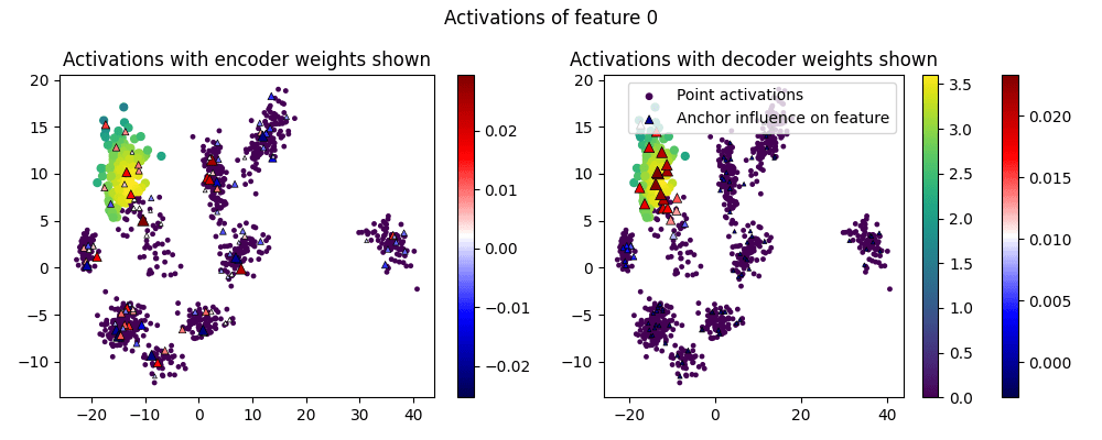
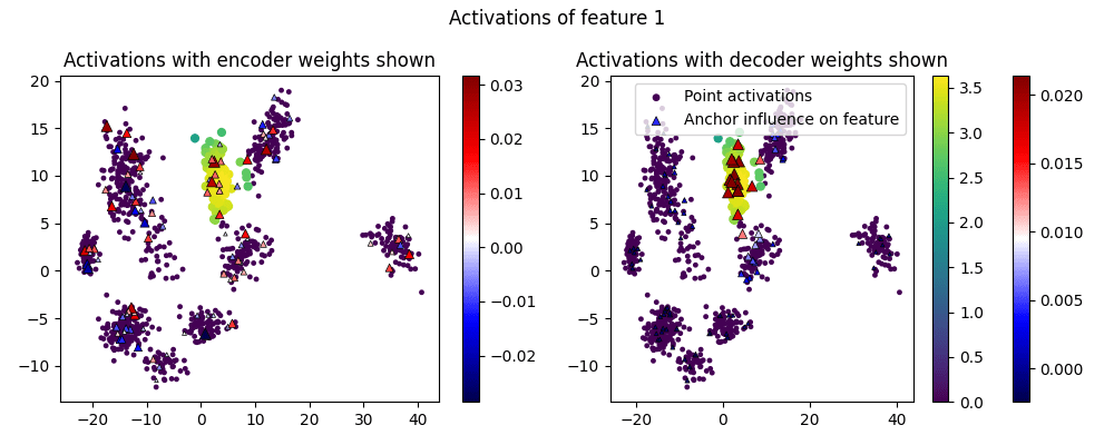
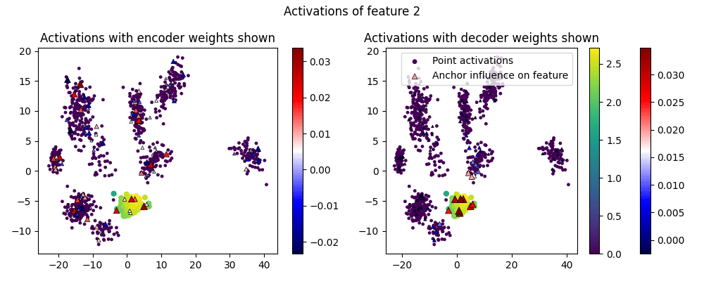
(I've omitted Features 3-9.)

One thing we can see is that the activations are larger in the center of the cluster, as we'd hope.

Another thing to notice is that the decoder weights are sparse and interpretable, as they activate the most within a cluster. But the encoder weights are all over the place - they are positive all across the dataset. We'll use this insight in the next section to fix the confused points.

[Edit 11/25: The non-interpretable encoder weights are actually an easy fix: use a small weight decay while turning off encoder normalization. This results in interpretable encoder AND decoder features, like so:]

Improving the Random Blobs result with "Adjoint Classification"

If you run the Random Blobs dataset with the scale parameter $\sigma =0.2$ (up from 0.11) which seemed best in the scale sensitivity experiment, and with $n_{anchors}=1000$ (up from 100), you get much better clustering results:

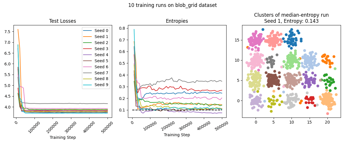
This is a big improvement, but we have huge number of "confused points", such as the single blue point in the upper-left which is closer to the pink clusters, but oddly gets assigned to the blue cluster.

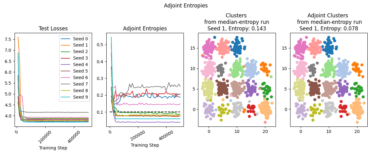
Seeing in the last experiment that decoder weights are more interpretable, I was inspired to try a process I call Adjoint Clustering: we assign clusters using the decoder weights via:

$cluster\left(p\right)=argmax(W_d^T\cdot embed(p\left)\right)$

where $p$ is a point and $W_d$ are the decoder weights.

By combining improved scale factor, increased number of anchors, and adjoint clustering, we get high-quality results even on the difficult Blob Grid dataset:

Takeaways for Sparse Autoencoder Research

Here are the components of this research that I hope generalize to other uses of SAEs:

1. You can use SAEs for other tasks besides interpreting language models! This is obviously not news, since SAEs were invented before language models, but its worth remembering.
2. You can train your SAE on the same data for many epochs. In my original training setup, I used 1e5 data, but by drastically increasing the number of epochs, I was able to get a Pareto improvement in both data requirements and performance. This may be because my underlying distribution is relatively simple, but I think its worth trying on language data too, or in any place where data is expensive to produce. A good experiment would be decreasing data by 1 OOM while increasing training epochs by 1 OOM.
3. We can validate SAEs on language models by checking for features in other fields. Something that keeps me up at night is that the interpretability of SAEs is just an illusion [LW · GW], as I've written about before [LW · GW]. I think experiments like this serve as a "training ground" where we can find what SAE architectures and flourishes are needed to find known features.
4. An alternative Ghost Grad. My version of the ghost gradient might be worth trying elsewhere. Its main benefit is that it does not require a second forward pass (it is computed just from $x$ and $\tilde{x}$), and that it aggressively resurrects features [make a graph showing this]. That said, it may be too simple or too specialized to work in other cases.
5. Adjoint Interpretation. I found that my encoder weights were far less interpretable than my decoder weights, and I got better performance at the target clustering task by interpreting $W_d^{T}x$ rather than $W_{e}x$.

Limitations and Future Work

1. All my datasets are artificial. I have some real data to try this on next.
2. I haven't done enough baselining: do SAEs outperform DBSCAN? Is the point cloud embedding"doing all the work"?
3. I have chosen the two main hyperparameters, $\sigma$ and $n_{features}$, manually. While we've seen that $\sigma$ has a range of reasonable values, my method for finding the correct $n_{features}$ is not reliable.
4. While decoder directions are interpretable, encoder directions are not. Why? Is there a way to fix this? I've tried tied weights (didn't work) and weight decay (scales everything down, including the anchors which should be active). [Edit 11/25: This was actually an easy fix: a small weight decay is sufficient, but was previously ineffective because I was normalizing the encoder. Turning off encoder normalization results in interpretable encoder weights.]
5. I've tried this approach with Anthropic-style SAEs, but with less success. It is not clear this technique can work without the in-built $k=1$ sparsity.

Code

My code is available at https://github.com/RobertHuben/point_cloud_sae/tree/main (currently poorly documented).

Acknowledgements

Thanks to Andrew and Logan for their comments on an early draft.

1. ^{^}

   I've tried ReLU, exp, and the identity function as alternatives to softplus. Softplus performs the best in my initial tests.

2. ^{^}

   The diagrams in this report show results on the test set, which also consists of 1000 points.

3. ^{^}

   For a full description, see "Data Clustering: Algorithms and Applications" by Charu C. Aggarwal and Chandan K. Reddy, page 574.

0 comments

Comments sorted by top scores.