The Internal Model Principle: A Straightforward Explanation

post by Alfred Harwood · 2025-04-12T10:58:51.479Z · LW · GW · 1 comments

Contents

  Two Sentence Summary
  The Setup
  The Punchline of the IMP
  The Assumptions of the IMP
    Assumptions regarding the basic setup
    Assumptions regarding the set of 'desirable states'
    The Detectability Condition
    The Feedback Structure Condition
  Proof of the IMP
      Theorem Part 1:
      Theorem Part 2:
      Theorem Part 3:
  How is the controller 'modelling' the environment?
  Conclusion
None
1 comment

This post was written during the Dovetail research fellowship. Thanks to Alex [LW · GW], Dalcy [LW · GW], and Jose [LW · GW] for reading and commenting on the draft.

The Internal Model Principle (IMP) is often stated as "a feedback regulator must incorporate a dynamic model of its environment in its internal structure" which is one of those sentences where every word needs a footnote. Recently, I have been trying to understand the IMP, to see if it can tell us anything useful for understanding the Agent-like Structure Problem [LW · GW]. In particular, I was interested whether the IMP can be considered as selection theorem [LW · GW]. In this post, I will focus on explaining the theorem itself and save its application to the Agent-like Structure Problem for future posts^[1]. 

I have written this post to summarise what I understand of the Internal Model Principle and I have tried to emphasise intuitive explanations. For a more detailed and mathematically formal distillation of the IMP, I recommend Jose's post [LW · GW] on the subject.

This post focuses on the 'Abstract Internal Model Principle' and is based on the paper 'Towards an Abstract Internal Model Principle' by Wonham and the first chapter of the book 'Supervisory Control of Discrete-Event Systems' by Wonham and Cai. There also exists a version of the IMP that is framed in the more traditional language of control theory (using differential equations, transfer functions etc.) which is described in  another paper, but I will not focus on it here. The authors imply that this version of the IMP is just a special case of the Abstract IMP but I haven't verified this. From now on, I will use the term 'IMP' to refer to the Abstract IMP.

The mathematical prerequisites for reading this post are roughly 'knows what a set is' and 'knows what a function is'^[2]. The paper and book chapter use a lot of algebraic formalism and lattice theory notation in order to look intimidating be mathematically rigourous. The book chapter is also used to introduce a lot of other concepts for use later in the book but which aren't strictly necessary for just understanding the IMP. I think that by sacrificing these elements we can buy a lot of clarity at the cost of very little rigour. By explaining the IMP in this way, I hope that we can see what it is actually saying, rather than being blinded by mathematical notation. 

Let's begin!

Two Sentence Summary

Before going through the proof, I will give a high-level two-sentence summary of the result so that you can see where it is going:

If we have two dynamical systems which jointly evolve and we enforce that one of them is autonomous, then there is some level of coarse-graining at which the two systems are isomorphic. If you call the autonomous system a 'controller' and the other system the 'environment' then you can say that this isomorphism is a 'model' and that the controller is 'modelling' the environment.

In this summary, the first sentence captures the mathematical theorem of the IMP and the second sentence captures its interpretation when applied to control theory, 

If this doesn't make sense to you, don't worry, I will explain it all in much more detail. If this does make sense to you and you can think of ways in which it is unsatisfactory, I probably agree with you^[3]. But, as stated earlier, this post is just intended to explain the result. I will not be discussing or arguing its usefulness here.

The Setup

There are two parts to the setup considered in the IMP, which I will call the 'environment' and the 'controller'. The original paper actually introduces a more fine-grained (and arguably more interesting) description of the setup, involving separate characterisations of the 'exosystem', 'controller' and 'plant' but as far as I can tell, these distinctions are abandoned shortly after they are introduced and they do not play any crucial role in the proof. As a result my description will just use the 'environment' and 'controller'. I will use the word 'system' to refer to the 'total' (ie. joint) environment-controller system.

The set of controller states is denoted $W$ and the set of joint environment-controller states is denoted $X$^[4]. For completeness, we might also want to describe the set of environment states as $S$, but surprisingly this set doesn't play much of a role in proof.

While we might want to represent the joint environment-controller state in some exotic way, a typical way is as a pair:

$$x=(s,w),$$

where $x\in X$, $s\in S$ and $w\in W$. We will use $\gamma :X\to W$ to denote the mapping which takes us from the joint pair to the controller state alone. Using the above representation, the mapping $\gamma$ is the projection:

$$\gamma (s,w)=w.$$

We assume that the joint environment-controller variable evolves according to an evolution rule given by the map $\alpha :X\to X$. Its worth briefly considering what it means for the joint environment-controller state to evolve deterministically according to a map. Note that, in this representation, there is no explicit 'action' taken by the controller which causes the system to evolve. Similarly, there is no explicitly causal effect of the system on the controller. Any effect that the controller has on the system (or vice versa) is bundled up into $\alpha$. Because of this, situations where the joint environment-controller state is the same, but the controller takes a different 'action' would be described by different $\alpha$ mapping. Implicitly, this formalism implies that the controller is pursuing a deterministic policy and that the environment responds deterministically to the controller.

This means that the joint system can be viewed as a discrete-time, deterministic, dynamical system. If we denote the system state at time $t$ as $x\left(t\right)$, the the system is governed by the evolution rule

$$x(t+1)=\alpha \left(x\right(t\left)\right).$$

The Punchline of the IMP

The main mathematical result of the IMP comes in the form of the following theorem(s). Suppose that the system dynamics are such that the joint environment-controller system always stays in a set of 'good' states. This is the criteria used to say whether the controller is doing a good job. If this is case then (subject to some important assumptions, discussed in the next section) the following hold:

1. There exists a unique map $\overline{\alpha }:W\to W$ which governs the autonomous evolution of the controller. This map is uniquely determined by $\gamma ,\alpha$ and the set of 'good' states $K\subset X$.
2. Let $X^{+}\subseteq K$ be the subset of good states where the system is kept. Then there is an injective (one-to-one) mapping ${\gamma }^{+}:X^{+}\to W$ between $X^{+}$ and the controller states. In other words, each good state in the set where the system remains has a unique controller state.
3. $\overline{\alpha }\circ {\gamma }^{+}={\gamma }^{+}\circ \alpha$. This condition means that, starting with a system state in $X^{+}$, finding the controller state using ${\gamma }^{+}$, then evolving that controller state through $\overline{\alpha }$ yields the same controller state as evolving the total system state through $\alpha$, followed by finding the corresponding controller state using ${\gamma }^{+}$. (Here the notation '$\circ$' means function composition so ${\gamma }^{+}\circ \alpha$ means 'applying $\alpha$ to an $x$-value, then applying ${\gamma }^{+}$ to the result'.)

One nice visual way that these results can be expressed is through a commutative diagram (don't worry, this isn't going to turn into a category theory post).

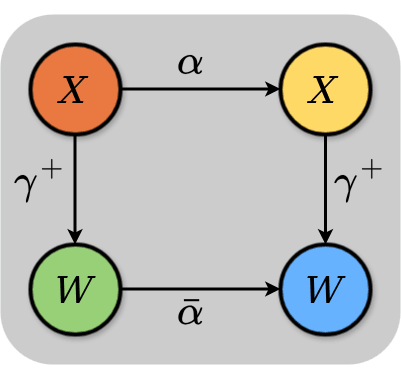
In this diagram, the nodes are sets and the directed edges are functions which map between the sets. Note that we can take two different 'routes' from the top left node to the bottom right node. We could pick an element in $X^{+}$ (the top left node) and evolve it using $\alpha$ (travelling across the top edge to the top right node), then use ${\gamma }^{+}$ to project out the controller value (travelling down the right hand edge to the bottom right node). Alternatively, you could start with an element in the top left node and first travel down the left hand edge of the diagram, projecting out a controller state through ${\gamma }^{+}$, before evolving that controller state using $\overline{\alpha }$ (travelling across the bottom edge) to get a new controller state, ending up in the bottom right node. We can say that this diagram 'commutes' which means that, starting from the same element of $X^{+}$ in the top left, both of these routes will result in the same controller value in the bottom right node.

Thus, every controller state corresponds to a unique system state, and you can track the evolution of the system solely by observing the evolution of the controller. In this sense, the controller is said to be 'modelling' the system. Or, as the authors put it: "an ideal feedback regulator will will include in its internal structure a dynamic model of the external ‘world’ behavior that the regulator tracks or regulates against". Unfortunately, this result comes at the cost of some pretty strong assumptions.

The Assumptions of the IMP

In equation (5) of paper, the mathematical assumptions underpinning the IMP are explicitly stated. Here, I will go through them one by one and explain the motivation behind them.  

A common theme in the following sections is that I'm going to explain the 'assumptions' of the paper as ways of defining $X$, $W$, etc. rather than assumptions as normally understood. This might seem unnecessary but I think its a lot clearer this way. Otherwise, it is quite easy to come up with systems (as characterised by a particular $(X,\alpha ,\gamma )$ set) which fail to meet the assumptions. But by slightly changing how you define the terms, you can still get the IMP to say something about the system.

Assumptions regarding the basic setup

First, some we will cover some basic 'assumptions' that are more like definitions of the basic setup (but they are included in the 'assumptions' section of the paper and it is useful to recap them here). 

• There exists a set of joint environment-controller states $X$
• There exists a set of controller states $W$
• There exists a 'joint evolution' function $\alpha :X\to X$
• There exists a mapping from each joint state to the corresponding controller state $\gamma :X\to W$.

So far, nothing too controversial. These have hopefully already been explained in the 'Setup' section above.

Assumptions regarding the set of 'desirable states'

The IMP states that, if the joint environment-controller system always stays within a set of 'good' (or 'desirable') states (which is a subset of all possible states), then (subject to further assumptions) the controller will contain an internal model of the environment (as described earlier). The next few assumptions/conditions involve characterising this set of good states.

• There exists a set $K$ of desirable environment-controller states which is a subset of $X$. So we have $K\subseteq X$ .
• There exists a subset $X^{+}$ of these desirable states $X^{+}\subseteq K$ where the controller will keep the system.
• Once the system enters the set $X^{+}$, it will stay there for all future timesteps.

We say that $X^{+}$ is $\alpha$-invariant ie. applying $\alpha$ to any member of $X^{+}$ will result in another state which is also a member of $X^{+}$. Since $X^{+}$ is a subset of the desirable states $K$, this is the way in which we formalise the fact that the controller keeps the system within the set of desirable states. The fact that $X^{+}$ is $\alpha$-invariant can be expressed by writing:

• $\alpha \left(X^{+}\right)\subseteq X^{+}$.

These definitions partially characterise the set of desirable states $K$ and the set of $\alpha$-invariant desirable states where the system is kept. There is another condition relating the set of desired states $K$ to the controller states $W$ which I will include here:

• The set of desired joint environment-controller states $K$ involves the full set of controller states $W$. This can be expressed by writing $\gamma \left(K\right)=W$. 

Wonham describes this condition as saying: "knowledge merely  that $x\in K$ ... yields no information about the control state $w\in W$". I don't particularly like this way of framing the condition. After all, it is pretty easy to come up with an example where a controller uses one set of states $W_1$ to steer the system into $K$ but once the system in in $K$, it only uses a different set of states $W_2$ to keep the system within $K$. In such a situation, we have$W=W_2\cup W_2$but $\gamma \left(K\right)=W_2\ne W$, so the condition isn't satisfied. I prefer to think of the $\gamma \left(K\right)=W$ as a definition of $W$. In this interpretation, the IMP is only concerned with the controller states that are 'activated' within the desired set of states. The controller might have millions of other possible states, but we are only concerned with the set $W:=\gamma \left(K\right)$ as these are the states that will be involved in the 'internal model' whose existence will be proved later.

The next two assumptions are the Detectability Condition and the Feedback Structure Condition, which both require a bit more explanation, so I have given them their own sections.

The Detectability Condition

This condition is phrased in the paper as:

• $X^{+}$ is detectable relative to $(\gamma ,\alpha )$.

What this means in practice can be explained fairly simply, but the mathematical conditions associated with formalising this claim are a bit more involved. Fortunately, a simple understanding is all you need to understand the proof of the IMP, so I will provide that. For readers more inclined towards formal mathematics, a more detailed explanation of how this condition is formalised is can be found in Jose's post [LW · GW] under the heading 'Observability Condition'^[5]. 

Imagine we had a system where the joint environment-controller state is $x_0\in X^{+}$. However, we cannot observe the full system state, we can only see what state the controller is in. In other words, we receive the observation $\gamma \left(x_0\right)=w_0\in W$. Now suppose that the full system is allowed to evolve through $\alpha$, generating a series of joint controller-environment states:

$$x\left(0\right)=x_0,x\left(1\right)=\alpha \left(x_0\right),x\left(2\right)=\alpha \left(\alpha \right(x_0\left)\right)x\left(3\right)=\alpha \left(\alpha \right(\alpha \left(x_0\right)\left)\right)...etc.$$

Recall that we are using $x\left(t\right)$ to indicate the joint controller-environment state at time $t$. In general $x(t+1)=\alpha \left(x\right(t\left)\right)$.

Now imagine that we are restricted to only viewing the corresponding controller states:

$$w\left(0\right)=w_0,w\left(1\right)=\gamma \left(x\right(1\left)\right),w\left(2\right)=\gamma \left(x\right(2\left)\right),...w\left(t\right)=\gamma \left(x\right(t\left)\right).$$

We can then ask the following question: if we had full knowledge of $\alpha$ and $\gamma$ and received this (potentially infinite) sequence of controller states, could we identify the full environment-controller state $x_0$ where the system started? Assume that we know that the system has started in $X^{+}$ but we don't know the exact state. 

If, for a particular $\alpha$ and $\gamma$ the answer to this question is 'yes' for all states in the set $X^{+}$, then we say that $X^{+}$ is detectable with respect to $(\gamma ,\alpha )$.

What is the motivation behind requiring this condition? As with some of the other conditions, I think that this is better understood as a condition on how we define $X^{+}$. 

Imagine that $X^{+}$ failed to satisfy the Detectability Condition. Let $Z\left(x\right)$ denote the sequence of controller states generated by starting the system in state $x$ and evolving it according to $\alpha$. Then, if $X^{+}$ failed to satisfy the Detectability Condition, we could find two $X$-values $x_a,x_b\in X^{+}$ which produced identical sequences ie. $Z\left(x_a\right)=Z\left(x_b\right)$. 

By definition, all states that start within $X^{+}$ will stay in $X^{+}$ regardless of the number of evolutions. This means that, in order to keep the system in the desired subset, the controller must perform exactly the same actions, regardless of whether the system started in state $x_a$ or $x_b$. Anthropomorphising a little, from the point of view of the controller, there is no practical difference between $x_a$ and $x_b$. So if we have a system which does not satisfy the Detectability Condition, we are saying that there is at least one pair of system states that we have labelled as 'different' which, for all practical purposes are identical from the point of view of the controller. Requiring the Detectability Condition is satisfied is the same as saying that we only label states as 'different' if they actually result in different controller behaviour at some point down the line. 

By thinking of the condition in this way, we can see that if we had a system which did not satisfy the Detectability Condition, then we could re-label the system in such a way that it did satisfy the condition by only counting states as different if they resulted in different behaviour from the controller. In the example above, a system with both $x_a$ and $x_b$ would not satisfy the Detectability Condition, but the system could be made to satisfy the condition if we lumped the two states together to form a new state $x_c$. The system would be considered to be in state $x_c$ if it was in $x_a$ or $x_b$. Note that this process doesn't involve changing any important features of the system, only changing the way in which we label the states.

Remember that the final result of the IMP is to show that the controller is 'modelling' the environment. Considering the Detectability Condition in light of this fact, it seems reasonable. It would be unreasonable to require a controller to model the difference between two states which are indistinguishable to it. When considered in this way, the Detectability Condition ensures that the environment is defined such that the controller 'models' different states in the environment only insofar as they require different behaviour.

Understanding the Detectability Condition to the level described above is all that is required to understand the proof of the IMP. Though this concept is fairly intuitive, formalising it mathematically is surprisingly involved (at least, in the way that Wonham does it). Again, if you would like all of the details, a nice explanation can be found in Jose's post [LW · GW], under the heading 'Observability Condition'.

The Feedback Structure Condition

The final condition/assumption of the IMP is the 'Feedback Structure Condition'. As with the Detectability Condition, it has a fairly simple interpretation which can be explained in words and a slightly more involved mathematical formalisation. I find the motivation for this condition hardest to understand, so I've left it until last.

In words, the Feedback Structure Condition is as follows:

• While the system is in the set of desired states (ie. $x\in K$), the controller behaves autonomously. This means that the controller state $w(t+1)$ at time $t+1$ depends only on the previous controller state $w\left(t\right)$ and not on any other details of $x$.

Suppose we had two states $x_a,x_b\in K$ which both corresponded to the same controller state ie. $\gamma \left(x_a\right)=\gamma \left(x_b\right)=w_0$. Let the time evolution of these two states be denoted $y_a=\alpha \left(x_a\right)$ and $y_b=\alpha \left(x_b\right)$. Then the Feedback Structure Condition requires that $\gamma \left(y_a\right)=\gamma \left(y_b\right)$. 

If you are like me, upon hearing this assumption, you might have some questions. What is the motivation behind this assumption? And why is it called the 'Feedback Structure' condition when it doesn't seem to have anything to do with feedback? I don't think that these questions are addressed very clearly in the paper or book, so here is my attempt at answering them.

On the subject of the Feedback Structure condition, Wonham describes it as a formalisation of 'the assumption that the controller is actuated only when the system state deviates from the "desired" subset $K$' but doesn't really explain why this requires that the controller is autonomous within $K$, nor why this is a desirable quality for a controller to have, nor what this condition has to do with 'feedback structure'. Indeed, the first twenty times I read that sentence, it seemed to me that an autonomous controller of the kind specified above is doing the opposite of 'feedback', since it is in some sense 'ignoring' the environmental state.

To understand this, we need to understand the control theoretic model of a 'regulator' which Wonham used as an inspiration for the IMP: 

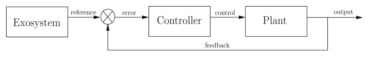
Here is Cai and Wonham's explanation of this diagram:

The objective of regulation is to ensure that the output signal coincides (eventually) with the reference, namely the system ‘tracks’. To this end the output is ‘fed back’ and compared (via ⊗) to the reference, and the resulting tracking error signal used to ‘drive’ the controller. The latter in turn controls the plant, causing its output to approach the reference, so that the tracking error eventually (perhaps as t → ∞) approaches ‘zero’.

Our aim is to show that this setup implies, when suitably formalized, that the controller incorporates a model of the exosystem: this statement is the Internal Model Principle.

Here is my translation of this, back into the terms of the Abstract IMP that we have been using in this post. There is some process by which the joint environment-controller state $x$ is compared to a 'reference' and the difference between the state and $x$ and the reference is used to generate a 'tracking signal'. In our case the 'reference' is the set of desired states $K$. If $x$ is not a desired state (ie. $x\notin K$), then the controller receives a signal from outside of itself that tells it to do something to move the system towards a desired state. However, if the system is already in a desired state then this 'tracking error' is zero. This means that the controller receives no signal from the outside world. As a result, the controller's state is the only thing that can affect its evolution while the system is in a desired state. This is why the assumption that the controller is 'actuated only when the system state deviates from the "desired" subset $K$' is equivalent to the controller behaving autonomously while in $K$.

As with the Detectability Condition, this simple understanding of the Feedback Structure Condition is all that is required to follow the proof of the IMP. If you would like the mathematical formalisation of this condition as used by Wonham, you can click on the collapsible section below to read some more details. But you can safely skip it if you just want to get to the proof.

More on the Feedback Structure Condition

The Feedback Structure Condition says that the controller must behave autonomously while the system is within the set of desired states. In the paper, this condition is described mathematically as follows:

$${\gamma }_K\le (\gamma \circ \alpha {)}_K.$$

What this inequality means and how it relates to the Feedback Structure Condition as we have described it requires a little bit of unpacking. In words, the above expression means the following: 'the equivalence relation induced by $\gamma$ (restricted to $K$) is finer than (or equal to) the equivalence relation induced by the composition of $\gamma \circ \alpha$ (restricted to $K$)'. 

The first thing to explain about this expression is that $\gamma$ and $\alpha$ are not taken to be the functions $\gamma$ and $\alpha$ that we introduced earlier. Here, they are taken to be the equivalence relations induced by those same functions. An equivalence relation is a way of chunking up (ie. partitioning) some set so that you say that elements in the same 'chunk' ('cell') are 'equal' in some sense. The equivalence relation induced by $\gamma$ is a way of partitioning the set $X$ so that all elements with the same value of $\gamma \left(x\right)$ are put in the same cell. Since $\gamma \left(x\right)$ is the controller state, the equivalence relation induced by $\gamma$ is the partition which divides up $X$ such that $x$-values with the same controller value occupy the same cell. So if $\gamma \left(x_a\right)=\gamma \left(x_b\right)$ for two different $x$-values, then we say that $x_a=x_b\left(\text{mod}\gamma \right)$.

Similarly, $\gamma \circ \alpha$ in the expression above corresponds to the equivalence relation induced by applying $\alpha$ and then $\gamma$ to an $x$-value. The condition that $\gamma \le \gamma \circ \alpha$ means that (the equivalence relation induced by) $\gamma$ is finer than (the equivalence relation induced by)  $\gamma \circ \alpha$. If one equivalence relation $E_1$ is 'finer' than another equivalence relation $E_2$, it means that, for any two elements $x_a$ and $x_b$, if $x_a=x_b\left(\text{mod}{E}_1\right)$ then $x_a=x_b\left(\text{mod}{E}_2\right)$. But if $x_a=x_b\left(\text{mod}{E}_2\right)$, this doesn't automatically imply that $x_a=x_b\left(\text{mod}{E}_1\right)$. This can be intuitively visualised by imagining two difference ways of partitioning a space, one of which is strictly finer than the other:

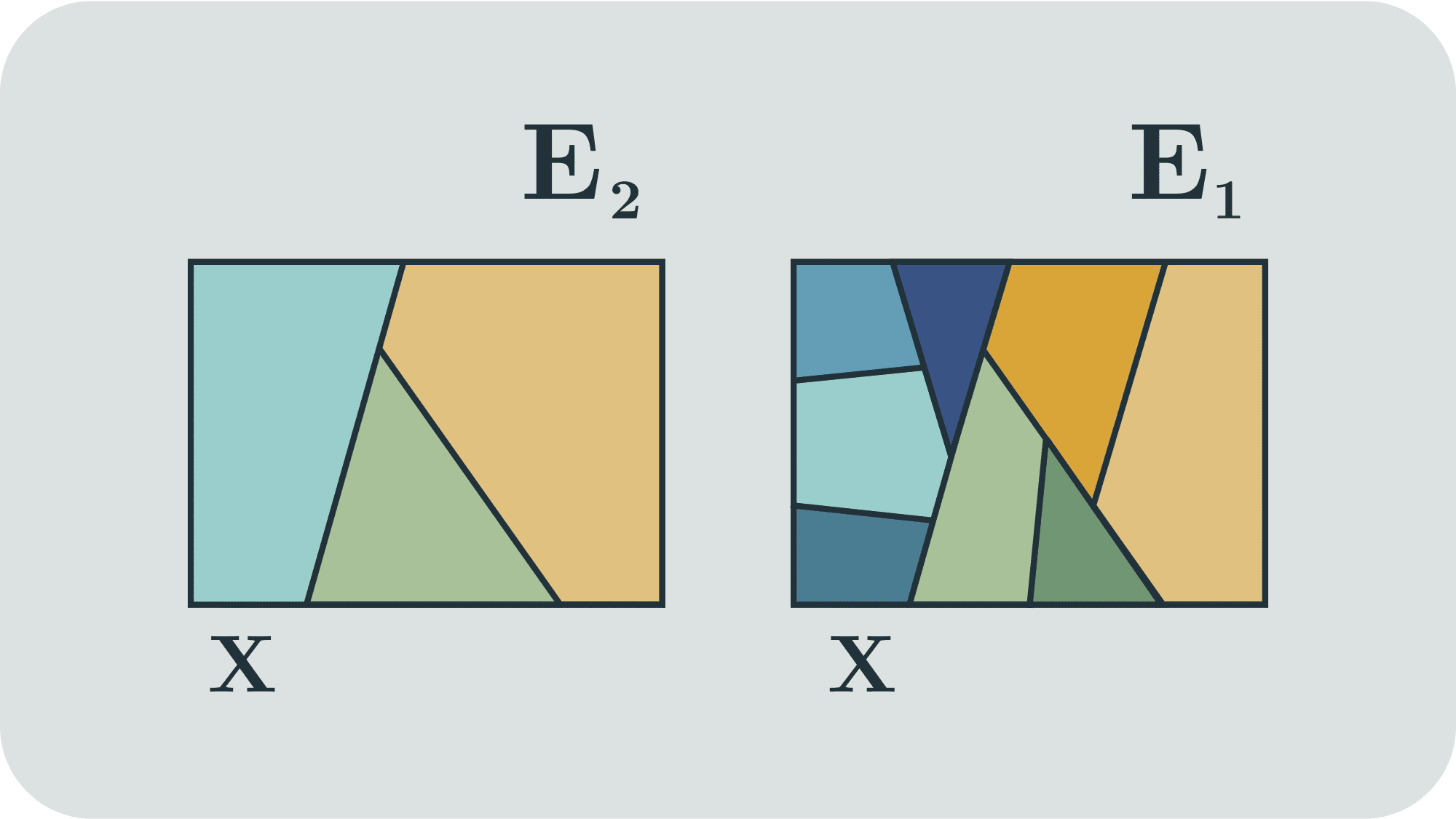
If we take any two elements in the dark green cell of $E_1$, then they will both be in the same cell according to $E_2$, because $E_1$ is finer than $E_2$. But if we take two elements of the green cell of $E_2$, that doesn't necessarily imply that they will be in the same cell of $E_1$, since one might be in the dark green cell and the other in the light green cell.

Finally, the '$K$' subscripts in the expression ${\gamma }_K\le (\gamma \circ \alpha {)}_K$ indicate that we are only considering these equivalence relations within the subset of desired states $K$.  We are now in a position to understand how this expressions relates to the condition that the controller is autonomous when restricted to the set of desired states.

The condition ${\gamma }_K<(\gamma \circ \alpha {)}_K$ means that if two $x$-values $x_a,x_b\in K$ have the same controller value (ie. $x_a=x_b\left(\text{mod}\gamma \right)$) then $\alpha \left(x_a\right)$ and $\alpha \left(x_b\right)$ will also have the same controller values (ie. $x_a=x_b(\text{mod}\gamma \circ \alpha )$). This is precisely the condition that we identified at the start of this section as being necessary for the controller to be autonomous within the set of desired states. With this, we have connected our initial understanding of the Feedback Structure Condition with its mathematical formulation ${\gamma }_K\le (\gamma \circ \alpha {)}_K$.

As with the other conditions discussed here, a more in-depth treatment of the Feedback Structure Condition can be found in Jose's post [LW · GW].

Proof of the IMP

We have now introduced all of the assumptions/conditions required for the IMP. To recap, we have:

• Joint environment-controller states $X$
• Controller states $W$
• The 'desired' subset $K\subset X$
• $\alpha :X\to X$
• $\gamma :X\to W$
• $\gamma \left(K\right)=W$
• Detectability: $X^{+}$ is detectable relative to $(\gamma ,\alpha )$
• Feedback Structure: ${\gamma }_K\le (\gamma \circ \alpha {)}_K$

Additionally, we will introduce some notation to denote the functions $\alpha$ and $\gamma$ when restricted to the set $X^{+}$. Often the restriction of a function to a smaller domain is denoted using a vertical bar, so the restriction of $\alpha$ to $X^{+}$ is denoted $\alpha |X^{+}$ and the restriction of $\gamma$ to the set $X^{+}$ is denoted $\gamma |X^{+}$. We will use the shorthand:

$${\alpha }^{+}:=\alpha |X^{+},{\gamma }^{+}:=\gamma |X^{+}.$$

Since the assumptions contain a lot of the meat of the IMP, the actual proof follows quite straightforwardly once we have them. The IMP Theorem is stated in three parts which we'll prove one at a time. 

Theorem Part 1:

There exists a unique map 

$$\overline{\alpha }:W\to W$$

determined by the condition 

$$\overline{\alpha }\circ \gamma |K=\gamma \circ \alpha |K.$$

We mentioned earlier when discussing the Feedback Structure Condition that the controller is autonomous within the set of good states, meaning that its evolution depends only on the previous controller state and not on other details of the system. This part of the theorem characterises the evolution of the controller alone when it is in the set of good states. The map $\overline{\alpha }$ is the evolution map acting on the set of controller states which determines this evolution when the system is in the set of good states.

Its easier to define $\overline{\alpha }$ first and then show that it satisfies the condition above. So here is how we can calculate $\overline{\alpha }\left(w\right)$, given $w\in W$.

• Find an $x_w\in K$ with $\gamma \left(x_w\right)=w$ . By our assumption $\gamma \left(K\right)=W$, there will always be such an $x$.
• Then evolve this $x$ value by $\alpha$, leading to $\alpha \left(x_w\right)$.
• Then apply $\gamma$ to $\alpha \left(x_w\right)$, and take $\overline{\alpha }\left(w\right):=\gamma \circ \alpha \left(x_w\right)$.

While this might seem like an odd way to define a map, it is actually well-defined and unique. Applying $\gamma \circ \alpha$ is well-defined, so the only part of the above procedure that we need to clarify in order to make $\overline{\alpha }$ well-defined and unique is the first section: the selection of $x_w$. If there are multiple elements $x\in K$ with $\gamma \left(x\right)=w$, which one do we choose? Thankfully, it doesn't matter. If we have $x_a,x_b\in K$ with $\gamma \left(x_a\right)=\gamma \left(x_b\right)=w$ then, after applying $\gamma \circ \alpha$, they will both correspond to the same controller value. This is enforced by the Feedback Structure Condition ${\gamma }_K\le (\gamma \circ \alpha {)}_K$. (In fact, as we will see in Part 3 of this theorem, within $X^{+}$ each controller value will correspond to a unique system state, so there will only be one $x_w\in X^{+}$ corresponding to each controller state. But we're getting ahead of ourselves!)

Therefore, whether we take an $x$-value and extract its controller value using $\gamma$, then evolve it using $\overline{\alpha }$ or we take that $x$-value, evolve it using $\alpha$, then apply $\gamma$ to extract the controller value, we will get the same result (provided that the $x$-value we chose was in $K$). This means that $\overline{\alpha }$ satisfies the condition $\overline{\alpha }\circ \gamma |K=\gamma \circ \alpha |K$ .

Theorem Part 2:

The second part of the theorem is the relation

$$\overline{\alpha }\circ {\gamma }^{+}={\gamma }^{+}\circ {\alpha }^{+}.$$

I'm not quite sure why this result is given its own section. It follows straightforwardly from the previous section. We have just shown that 

$$\overline{\alpha }\circ \gamma |K=\gamma \circ \alpha |K.$$

Since $X^{+}\subseteq K$, this relation will also hold for all values in $X^{+}$. So we can replace $K$ with $X^{+}$ in this expression and then use our definitions of ${\gamma }^{+},{\alpha }^{+}$ (the restrictions of $\gamma$ and $\alpha$ to $X^{+}$) to obtain the expression:

$$\overline{\alpha }\circ {\gamma }^{+}={\gamma }^{+}\circ {\alpha }^{+}.$$

Done!

Theorem Part 3:

• ${\gamma }^{+}$ is injective

This means that for every $x\in X^{+}$, ${\gamma }^{+}\left(x\right)$ maps to a unique controller value in $W$. This follows from the Detectability and Feedback Structure conditions. We will prove this by contradiction.

Assume that there are two distinct elements $x_a,x_b\in X^{+}$ such that ${\gamma }^{+}\left(x_a\right)={\gamma }^{+}\left(x_b\right)=w_0$ (recall that ${\gamma }^{+}$ is just $\gamma$ restricted to $X^{+}$). In words, this means that there are two $x$-values in $X^{+}$ which correspond to the same controller state. If this was true, then ${\gamma }^{+}$ would not be injective. Now, by the Feedback Structure Condition, for both of these states, the controller will evolve autonomously, depending only the controller value $w_0$. This means that the subsequent controller states for $x_a$ and $x_b$ would be the same. Furthermore, every subsequent controller state from then on would be the same, whether the system started in $x_a$ or $x_b$. But this would violate the Detectability Condition, which requires that two states should only be labelled as different if they result in distinct controller behaviour. Therefore, a system which obeys the Feedback Structure Condition and the Detectability Condition must have ${\gamma }^{+}$ injective. 

How is the controller 'modelling' the environment?

Until now, we haven't talked much about what the environment is doing on its own. We have just been discussing either the joint controller-environment state or the controller on its own. 

We have proved (given some important assumptions) that a controller which keeps the total system within a set of good states will:

1. Evolve autonomously according to unique map $\overline{\alpha }:W\to W$ which is determined by the condition $\overline{\alpha }\circ \gamma |K=\gamma \circ \alpha |K$
2. Have a state which is related to the 'total' system state by an injective map ${\gamma }^{+}$ (when restricted to the $\alpha$-invariant subset)

This means that the controller is an isomorphic to the system. If the joint system is represented by environment-controller pairs $(s,w)$, then ${\gamma }^{+}$ being injective means that no two pairs (within $X^{+}$) will have the same environment value $s$ or controller value $w$. This means that with appropriate re-labelling, each joint state can be indexed:

$$(s_1,w_1),(s_2,w_2),(s_3,w_3),...\text{etc.}$$

In this new re-labelled setup, the joint evolution is just simply

$$\alpha (s_i,w_i)=(s_{i+1},w_{i+1})$$

The controller evolution is given by

$$\overline{\alpha }\left(w_i\right)=w_{i+1},$$

and the environment evolution is given by

$${\alpha }_E\left(s_i\right)=s_{i+1}.$$

The environment and the controller are isomorphic. This means that, if you know the controller state at time $t$, you can work out the environment state at time $t$ and all subsequent times. In this sense the controller is modelling the environment and, conversely, the environment is modelling the controller.

Conclusion

Hopefully, you now understand the Internal Model Principle better than you did before. Certainly, the process of writing this has helped me understand it more. There are lots of other things I want to talk about. Does the IMP work as a selection theorem? Do the assumptions carry over from feedback regulators to general agents? Does the concept of a 'model' used in the IMP correspond in any way to our notion of a 'world model' in agents? I think that the short answer to all of these questions lies somewhere between 'sort of' and 'no', but this post is already long, so I will save those for another day.

 

1. ^{^}

   This post is not intended as IMP apologetics. I won't be making the case that the IMP is 'useful' for the Agent-like Structure Problem (or anything else). I actually think that the IMP has some serious issues which require more discussion. But understanding the theorem is necessary to understand these issues so I have written this post first. At some point in the future, I might write up my criticisms in a future post.

2. ^{^}

   For example, if you understand the following notation then you probably have an appropriate level of mathematical skill to read this post:

   1. $A\subset B$ can mean '$A$ is a subset of $B$' 

   2.  $a\in A$ can mean '$a$ is an element of set $A$'

   3. $f:A\to B$ can mean '$f$ is a function which maps elements of set $A$ to elements of set $B$', 

3. ^{^}

   Here's one issue that you might already have noticed. One can always coarse-grain both controller and environment so that they each have only one state. If both controller and environment have only one state, then they are trivially isomorphic. In this sense, the IMP might seem trivial. In the IMP, the level of coarse graining is specified by the 'Detectability Condition' (discussed later in this post). In some systems, this coarse graining does result in the trivial isomorphism, but thankfully this is not the case for all systems.

4. ^{^}

   In this respect, (and most other respects) the notation used in this post follows the 1976 paper, which has some slight differences from the book chapter (eg. the book chapter uses $X_C$ to denote the set of controller states, instead of $W$).

5. ^{^}

   In this post I am following the terminology used in the 1976 paper. In the paper, 'observability' is a property of the $\alpha ,\gamma$ pair and a 'detectability' is a property of a set (eg. $X^{+}$) whose elements are acted on by $\alpha$ and $\gamma$. Jose's post, which is based more on the book chapter, uses the term 'Observability Condition' to mean the same thing as our 'Detectability Condition' in this post.

1 comments

Comments sorted by top scores.