Proof Explained for "Robust Agents Learn Causal World Model"

post by Dalcy (Darcy) · 2024-12-22T15:06:16.880Z · LW · GW · 0 comments

Contents

  Recalling the Basic Setup
    Assumptions
  Proof of the Exact Case
    Load-Bearing part of Oracle Use
    Identification via Induction
      Constraint 1: σ will remove D's parents
      Constraint 2: σ fixes the environment variables other than those in the path.
      Constraint 3: Let σ contain a local intervention making Ck a binary variable
  Proof of the Approximate Case
    New Assumptions
    Load-Bearing part of Oracle Use
    Identification via Induction
    Identifying the Approximate Graph Structure
None
No comments

This post was written during Alex Altair's agent foundations fellowship program [LW · GW], funded by LTFF. Thank you Alex Altair [LW · GW], Alfred Harwood [LW · GW], Daniel C [LW · GW] for feedback and comments.

This is a post explaining the proof of the paper Robust Agents Learn Causal World Model in detail. Check the previous post [LW · GW] in the sequence for a higher-level summary and discussion of the paper, including an explanation of the basic setup [LW · GW] (like terminologies and assumptions) which this post will assume from now on.

Recalling the Basic Setup

Let's recall the basic setup (again, check the previous post [LW · GW] for more explanation):

1. [World [LW(p) · GW(p)]] The world is a Causal Bayesian Network $G$ over the set of variables corresponding to the environment $C$, utility node $U$, and decision node $D$. The differences from a normal Causal Bayesian Network is that (1) $U$ is a deterministic function of its parents $U\left({Pa}_U\right)$, and (2) $P(D\mid {Pa}_D)$, the conditional probability distribution for $D$, is undetermined—it's something that our agent will select.
2. [Agent as a Policy Oracle [LW · GW]] An agent is a policy oracle ${\Pi }_{\Sigma }$ which is a function that takes in an intervention $\sigma \in \Sigma$ (where $\Sigma$ represents the set of all allowed interventions over $C$) and returns a policy ${\pi }_{\sigma }(D\mid {Pa}_D)$.
3. [Robustness as  [LW · GW]$\delta$-optimality under interventions [LW · GW]] We define a "robust" agent as a policy oracle whose regret is bounded by $\delta$ under some class of interventions over the environment $\Sigma$.

Assumptions

Also recall the following assumptions [LW(p) · GW(p)]:

1) Unmediated Decision Task states that ${Des}_D\cap {Anc}_U=\varnothing$. This is pretty major.

2) Domain dependence states that there exists distributions over the chance variables $P\left(C\right)$ and $P^{\prime }\left(C\right)$ (compatible with $M$) such that $\arg {max}_{\pi }{E}_P^{\pi }\left[U\right]\ne \arg {max}_{\pi }{E}_{P^{\prime }}^{\pi }\left[U\right]$.

• This is very reasonable. If domain dependence does not hold, then the optimal policy is just a constant function.

These together imply:

1. There does not exist a decision $d\in \mathrm{dom}\left(D\right)$ that is optimal, i.e. $\arg {max}_{d}U(d,x)$ across all $x\in X={Pa}_U\setminus \left\{D\right\}$.
2. $D\in {Pa}_U$, i.e. there can't be any intermediate nodes between $D$ and $U$, and all causal effects from $D$ to $U$ must be direct.

Now, with the basic setup of the paper recalled, let's prove the main theorems.

Proof of the Exact Case

We will first prove Theorem 1:

For almost all worlds $(G,P)$ satisfying assumption 1 and 2, we can identify the directed acyclic graph $G$ and the joint distribution $P$ over all variables upstream of $U$, given that we have access to a $0$-optimal policy oracle.

I will attempt to present the proof in a way that focuses on how one could've discovered the paper's results by themselves, emphasizing intuitions and how trying to formalize them naturally constrains the solutions or assumptions we must use.

Load-Bearing part of Oracle Use

Somehow we're going to have to elicit information out of the policy oracle.

Recall that the oracle is a function that maps an intervention to a policy, which is a conditional probability distribution ${\pi }_{\sigma }(D\mid {Pa}_D)$. It can be shown that if the oracle is optimal, this distribution is (almost always) a deterministic map. The argument goes like:

• Suppose that given a context ${Pa}_D={pa}_D$, two decisions $d$ and $d^{\prime }$ have the same expected utility.
• Then, we can argue that this is extremely unlikely:
  • Intuitively because exact equality is very unlikely for real number things.
  • More rigorously because expressing this equality results in a polynomial constraint over the parameters, which has Lebesgue measure 0 over the parameterization of the conditional probability distribution).
• Therefore it is extremely likely (probability 1) that there is a strict ordering of decisions (according to their expected utility) given a context, i.e. almost always a unique maximum EU decision given a context. Therefore an optimal policy must only choose that decision in that given context, i.e. deterministic.

Then, somehow our information-eliciting procedure is going to have to exploit the fact that, given a ${Pa}_D={pa}_D$, as we change the intervention $\sigma$, the optimal decision prescribed changes from $d$ to $d^{\prime }$.

To make this possible, we want to rule out the existence of a decision that is universally optimal across all inputs to the utility node, because then no intervention would yield a change in the output of the oracle.

• In math, a $d\in \mathrm{dom}\left(D\right)$ such that for all possible inputs $x$ to the utility (other than the decision), $d$ is always the $\mathrm{argmax}$ of $U(d,x)$, i.e. $d\in {\mathrm{argmax}}_{d}U(d,x)\forall x\in \mathrm{dom}\left(X\right)$ where $X={Pa}_U\setminus \left\{D\right\}$

Recall the first consequence of the two assumptions we had: There does not exist a decision $d\in \mathrm{dom}\left(D\right)$ that is optimal, i.e. $\arg {max}_{d}U(d,x)$ across all $x\in X={Pa}_U\setminus \left\{D\right\}$.

This implies that there is at least one $x^{\prime }$ where the optimal decision $d^{\prime }$ differs from $d$!

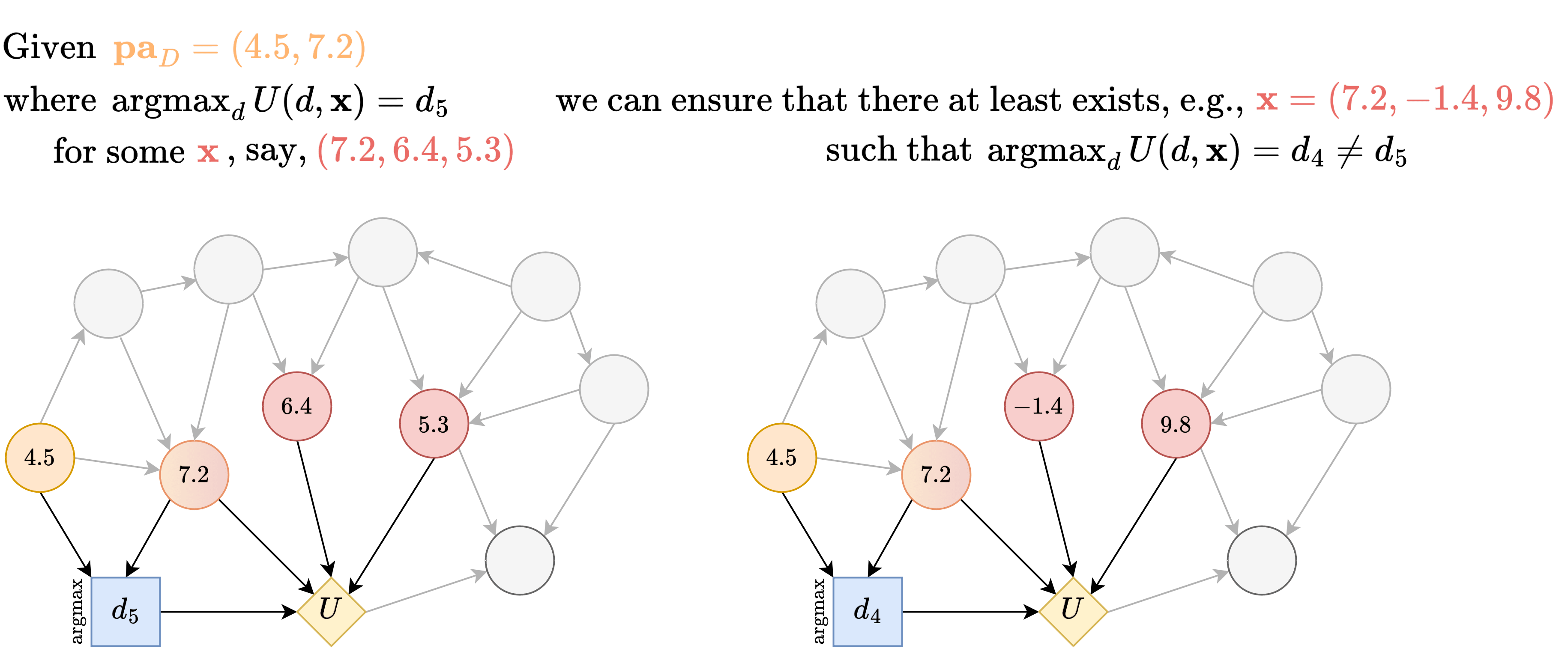
But the worry is that such $x^{\prime }$ will be incompatible with ${Pa}_D={pa}_D$.

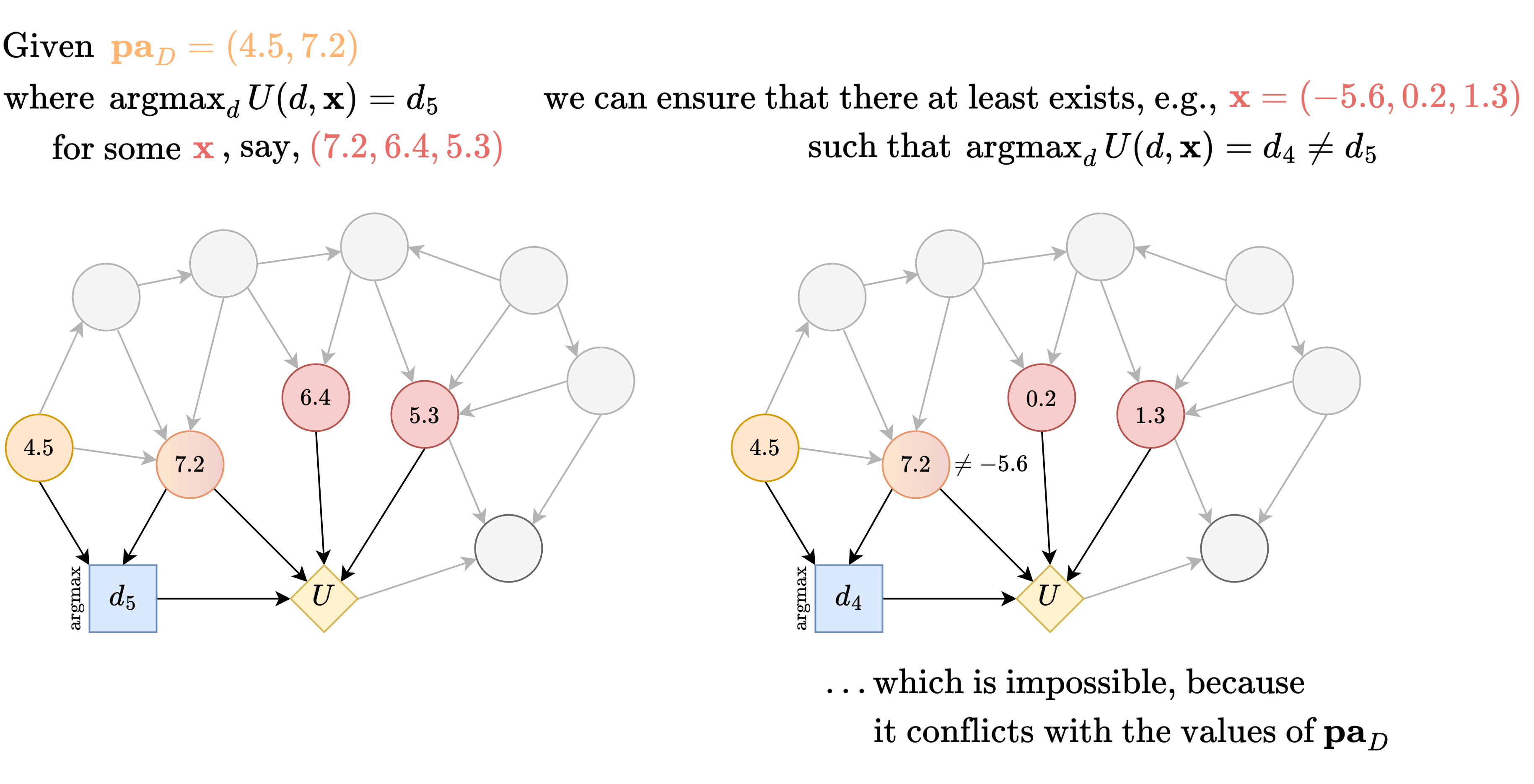
So, we will restricted to only considering $\sigma$ that masks the inputs of $D$ by only letting $D$ depend on ${P{a}^{\prime }}_D\subseteq {Pa}_D$ such that ${P{a}^{\prime }}_D\cap {Pa}_U=\varnothing$.

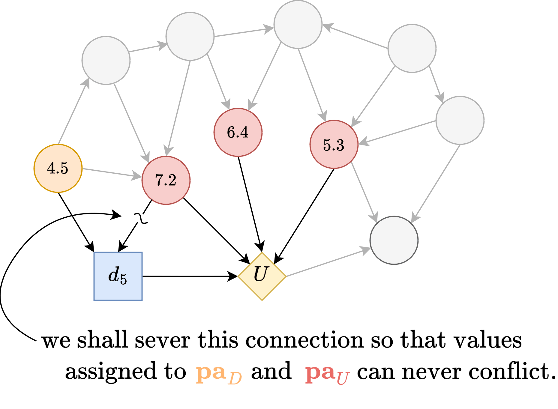
Then, given $\sigma$, let $d_1$ denote the optimal decision associated with some ${P{a}^{\prime }}_D={p{a}^{\prime }}_D$. Then, by the earlier argument, if we consider any intervention ${\sigma }^{\prime }$ that does $do(X=x^{\prime })$, then it would have a different optimal decision, call it $d_2$.

And to operationalize "as we change the intervention," we define a mixed local intervention $\tilde{\sigma }\left(q\right)=q\sigma +(1-q){\sigma }^{\prime }$.

When $q=0$, the policy oracle (under ${P{a}^{\prime }}_D={p{a}^{\prime }}_D$) would prescribe $d_1$, and for $q=1$, it would prescribe $d_4$. There may of course be other intermediate optimal decisions along the way as you slowly increase $q$ from $0$ to $1$ - say, $d_2$ and $d_3$ for the current example.

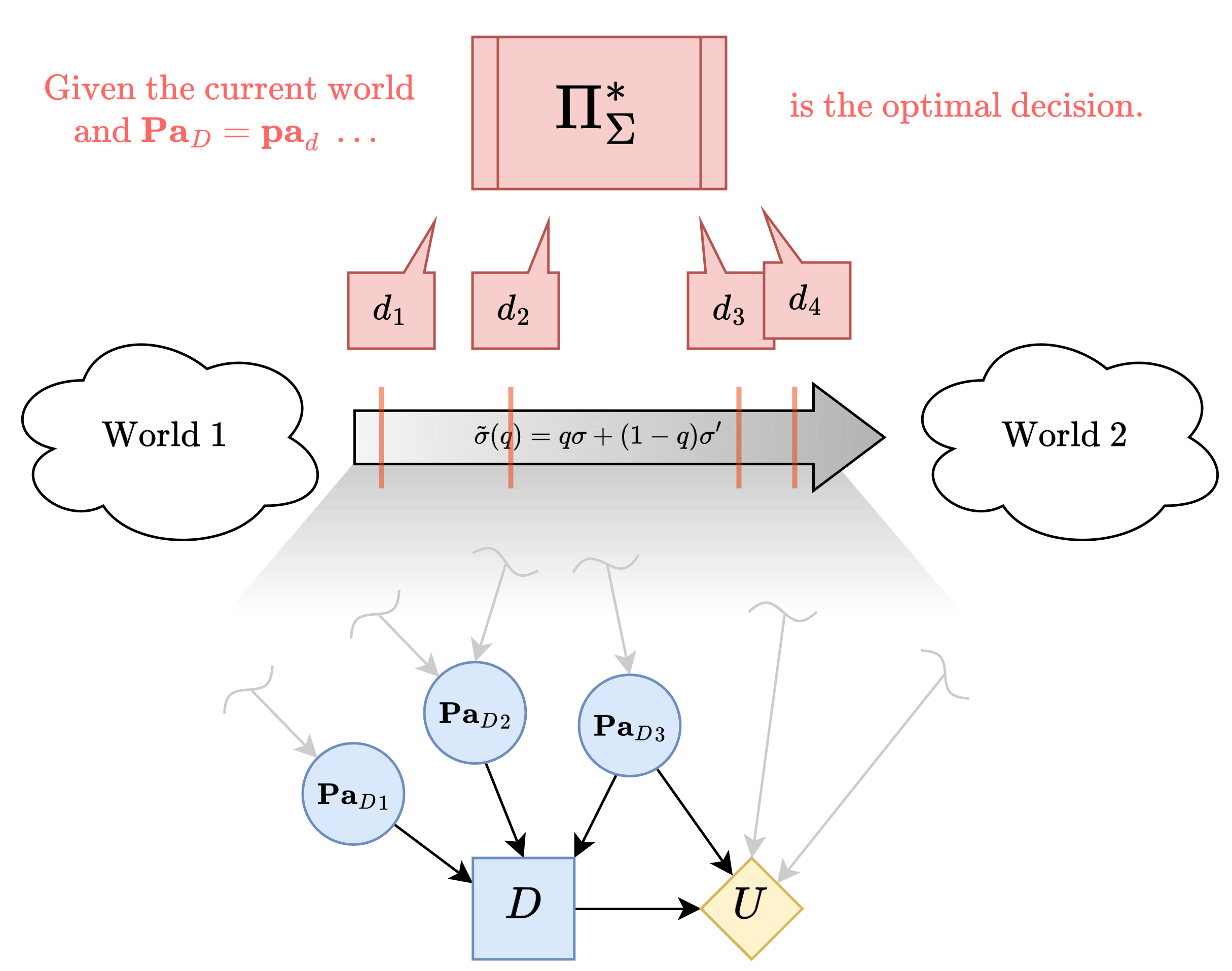
Note that once you switch your decision from $d$ to $d^{\prime }$ as you increase $q$, you will never encounter $d$ again because of linearity of $E[U\mid p{a}_D,\mathrm{do}(D=d);\tilde{\sigma }(q\left)\right]$. Namely:

$\begin{array}{cc}E[U\mid {pa}_D,\mathrm{do}(D=d),\tilde{\sigma }(q\left)\right]& =qE[U\mid {pa}_D,\mathrm{do}(D=d),\sigma ]\\ & +(1-q)E[U\mid {pa}_D,\mathrm{do}(D=d),\tilde{\sigma }]\\ & =q{U}_1+(1-q)U_2\\ & =U_2+q(U_1-U_2).\end{array}$

The diagram below makes it more clear why linearity implies the same decision never gets chosen twice. The oracle can be thought of as attaining the upper envelope, as denoted in dotted line.

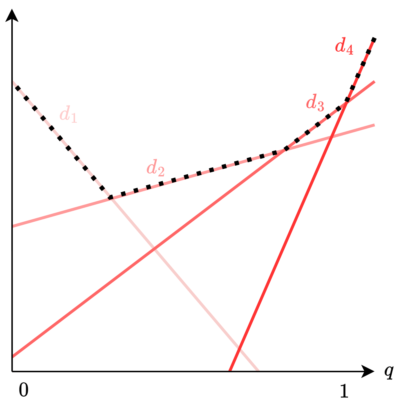
Let $q_{\text{crit}}$ represent the value of $q$ at which the optimal decision switches from some $d_3$ (may or may not be $d_1$) to $d_4$.

Insight: $q_{\text{crit}}$ is interesting. It's a behavioral property of our oracle, meaning we can estimate it by repeatedly sampling it (across random samples of $q\in [0,1]$). But it can also probably be expressed in closed-form in terms of some parameters of the environment (by just expanding out the definition of expected utility). So $q_{\text{crit}}$ is a bridge that lets us infer properties about the environment from the oracle.

Let's derive a closed-form expression of $q_{\text{crit}}$. Let $R=C\setminus {P{a}^{\prime }}_D$.

Detailed Proof

$q_{\text{crit}}$ is a value that satisfies$\begin{array}{cc}E[U|{p{a}^{\prime }}_D,\mathrm{do}(D=d_3);\tilde{\sigma }(q_{\text{crit}}\left)\right]& =E[U|{p{a}^{\prime }}_D,\mathrm{do}(D=d_4);\tilde{\sigma }(q_{\text{crit}}\left)\right]\end{array}$

Expanding out the left-hand side:$\begin{array}{cc}E[U|{p{a}^{\prime }}_D,\mathrm{do}(D=d_3);\tilde{\sigma }(q_{\text{crit}}\left)\right]& =\frac{1}{P({p{a}^{\prime }}_D;\tilde{\sigma }(q_{\text{crit}}\left)\right)}\sum _{r}U(d_3,x)P(r,{p{a}^{\prime }}_D;\tilde{\sigma }(q_{\text{crit}}\left)\right)\\ & =\frac{1}{P({p{a}^{\prime }}_D;\tilde{\sigma }(q_{\text{crit}}\left)\right)}\sum _{r}U(d_3,x)\left[q_{\text{crit}}P\right(r,{p{a}^{\prime }}_D;\sigma )+(1-q_{\text{crit}}\left)P\right(r,{p{a}^{\prime }}_D;{\sigma }^{\prime }\left)\right]\end{array}$

Expanding out the difference of both sides and setting it to zero:

$E[U|{p{a}^{\prime }}_D,\mathrm{do}(D=d_3);\tilde{\sigma }(q_{\text{crit}}\left)\right]-E[U|{p{a}^{\prime }}_D,\mathrm{do}(D=d_4);\tilde{\sigma }(q_{\text{crit}}\left)\right]$
$\begin{array}{cc}& =\frac{1}{P({p{a}^{\prime }}_D;\tilde{\sigma }(q_{\text{crit}}\left)\right)}\sum _r\begin{array}{cc}& q_{\text{crit}}P(r,{p{a}^{\prime }}_D;\sigma )\left[U\right(d_3,x)-U(d_4,x\left)\right]\\ & +(1-q_{\text{crit}})P(r,{p{a}^{\prime }}_D;{\sigma }^{\prime })\left[U\right(d_3,x)-U(d_4,x\left)\right]\end{array}\\ & =0\end{array}$

Now we solve for $q_{\text{crit}}$:$\begin{array}{cc}\sum _r{q}_{\text{crit}}P(r,{p{a}^{\prime }}_D;\sigma )\left[U\right(d_3,x)-U(d_4,x\left)\right]& =-(1-q_{\text{crit}})\sum _{r}P(r,{p{a}^{\prime }}_D;{\sigma }^{\prime })\left[U\right(d_3,x)-U(d_4,x\left)\right]\\ & =-(1-q_{\text{crit}})\left[U\right(d_3,x^{\prime })-U(d_4,x^{\prime }\left)\right]\end{array}$

$\begin{array}{cc}\frac{q_{\text{crit}}}{1-q_{\text{crit}}}& =\frac{-\left[U\right(d_3,x^{\prime })-U(d_4,x^{\prime }\left)\right]}{{\sum }_{r}P(r,{p{a}^{\prime }}_D;\sigma )\left[U\right(d_3,x)-U(d_4,x\left)\right]}\end{array}$

$\begin{array}{cc}{q}_{\text{crit}}& ={(1-\frac{{\sum }_{r}P(r,{p{a}^{\prime }}_D;\sigma )\left[U\right(d_3,x)-U(d_4,x\left)\right]}{U(d_3,x^{\prime })-U(d_4,x^{\prime })})}^{-1}\end{array}$

$\begin{array}{cc}{q}_{\text{crit}}& ={(1-\frac{{\sum }_{r}P(r,{p{a}^{\prime }}_D;\sigma )\left[U\right(d_3,x)-U(d_4,x\left)\right]}{U(d_3,x^{\prime })-U(d_4,x^{\prime })})}^{-1}\end{array}$

Again, $q_{\text{crit}}$ can be estimated from sampling the oracle. We know the denominator because we assume the knowledge of $U$.

Therefore, the oracle lets us calculate ${\sum }_{r}P(r,{p{a}^{\prime }}_D;\sigma )\left[U\right(d_3,x)-U(d_4,x\left)\right]$, the difference in expected utility of some two decisions given some context.

Restating our chain of inquiry as a lemma:

(Lemma 4) Given $\sigma$ that masks the inputs such that ${P{a}^{\prime }}_D\cap {Pa}_U=\varnothing$, $\forall {p{a}^{\prime }}_D$ $\exists d,d^{\prime }$ such that we can approximate ${\sum }_{r}P(r,{p{a}^{\prime }}_D;\sigma )\left[U\right(d,x)-U(d^{\prime },x\left)\right]$, where $R=C\setminus {P{a}^{\prime }}_D$ and $X={Pa}_U\setminus \left\{D\right\}$.

Identification via Induction

By the Unmediated Decision Task assumption, we see that the ancestors of U look like the following. We notice that there are two types of paths to consider in our induction argument.

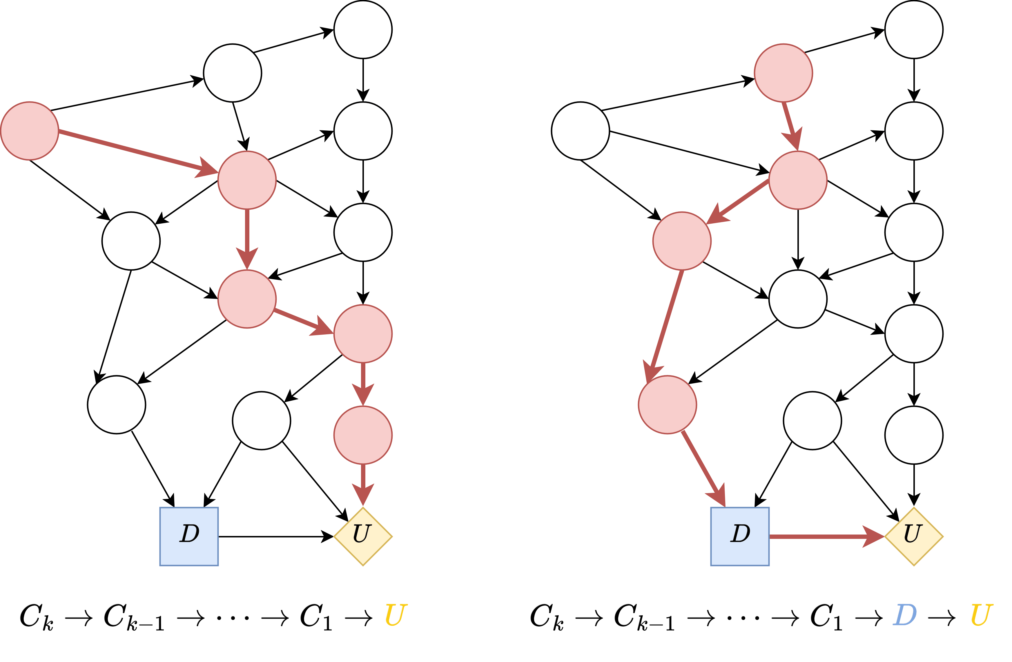
Let's first consider the first type, $C_k\to C_{k-1}\to \cdots \to C_1$, where $C_1\in {Pa}_U$, $C_1\ne D$.

We first define the following variables:

• $X={Pa}_U\setminus \left\{D\right\}$
• $Z={Anc}_U\setminus {Pa}_D$
• $R=C\setminus {P{a}^{\prime }}_D$
• $Y=C\setminus \{C_1,\dots ,C_k\}$

Assume ${Pa}_{k-1},\dots ,{Pa}_1$ are known, and $P\left(C_i|{Pa}_i\right)$ are known.

The claim to prove is that, given these are known, we can identify the conditional probability distribution $P\left(C_k|{Pa}_k\right)$.

Assume we have some $\sigma$. We want to identify $P\left(C_k|{Pa}_k\right)$, and we have to somehow use the policy oracle for that.

Recall from Lemma 4 that given an intervention $\sigma$ such that ${P{a}^{\prime }}_D\cap {Pa}_U=\varnothing$, for all values of ${p{a}^{\prime }}_D$, there exists two different decisions $d$ and $d^{\prime }$ such that ${\sum }_{r}P(r,{p{a}^{\prime }}_D;\sigma )\left[U\right(d,x)-U(d^{\prime },x\left)\right]$ can be identified.

The trick is in setting $\sigma$ such that it makes this sum contain $P(C_i=c_i|{Pa}_i={pa}_i)$ terms for all $1\le i\le k$, for arbitrary choices of $c_i$ and ${pa}_i$.

Let's think through how we might discover the right constraints on $\sigma$.

Constraint 1: $\sigma$ will remove $D$'s parents

Since we want ${P{a}^{\prime }}_D\cap {Pa}_U=\varnothing$, let's just choose $\sigma$ such that ${P{a}^{\prime }}_D=\varnothing$ hence $R=C\setminus {P{a}^{\prime }}_D=C$).

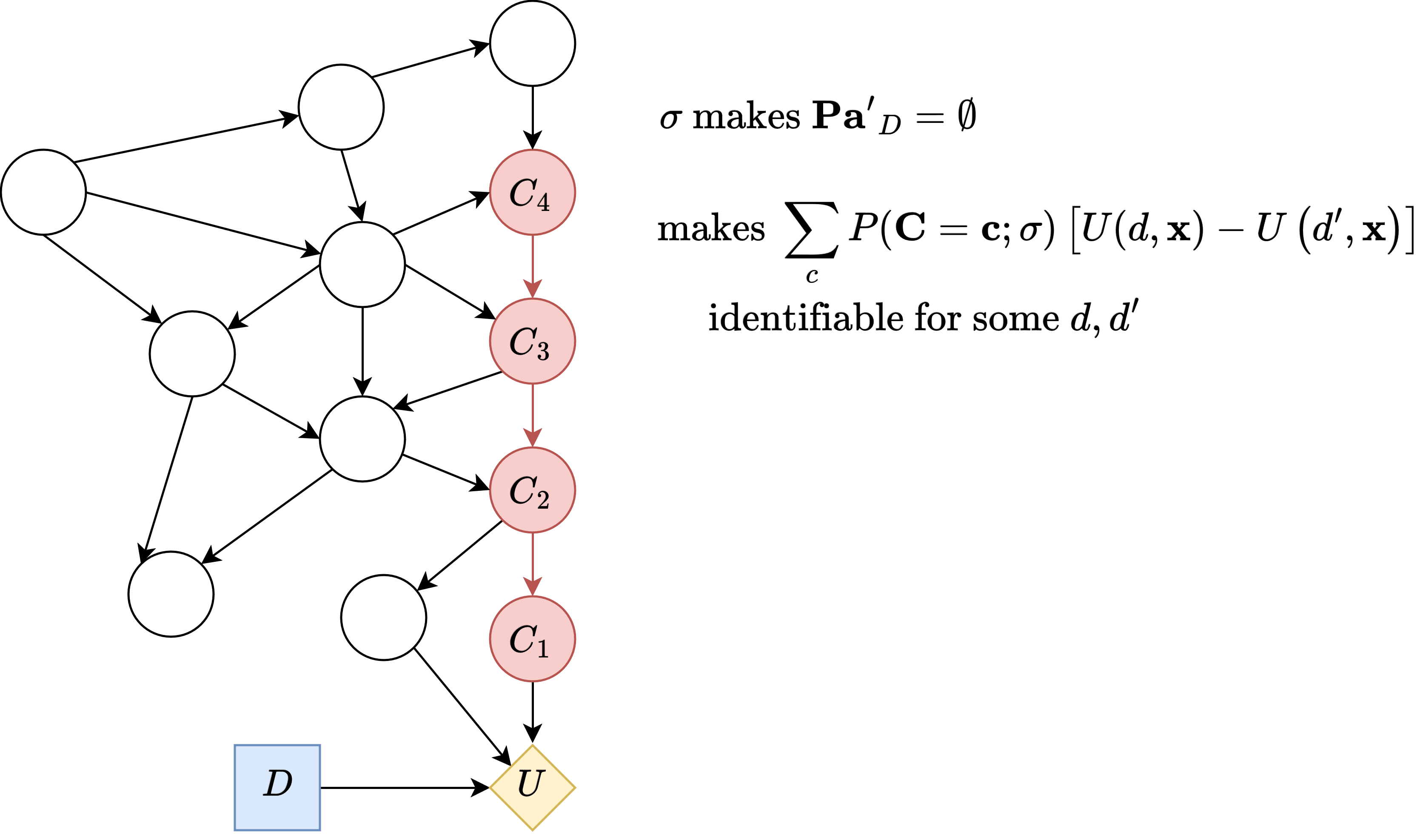
Constraint 2: $\sigma$ fixes the environment variables other than those in the path.

Note the following: Since ${\sum }_{c}P(c;\sigma )\left[U\right(d,x)-U(d^{\prime },x\left)\right]$'s value can be computed, if it can be expressed in terms of $P(c_1\mid p{a}_1)\dots P(c_{k-1}\mid p{a}_{k-1}),P(c_k\mid {pa}_k)$ that would let us solve for $P(c_k\mid {pa}_k)$, since by the induction hypothesis all the terms except it are known. Note that we also somehow have to figure out what the set ${Pa}_k$ is, too.

Expanding out the above sum will give us some clue as to what further constraints we must impose on $\sigma$ in order for the sum to be expressed that simply:

$\begin{array}{cc}P(C=c;\sigma )& =\prod _{C_j\in C}P(C_j=c_j|{Pa}_j={pa}_j;\sigma )\\ & =P(c_1|{pa}_1;\sigma )\dots P(c_k|{pa}_k;\sigma )\prod _{C_j\in Y}P(c_j|{pa}_j;\sigma )\end{array}$

How do we choose $\sigma$ such that
$\begin{array}{cc}\sum _{c}P(C=c;\sigma )[\ast ]& =\sum _c\left(P\right(c_1|{pa}_1;\sigma )\dots P(c_k|{pa}_k;\sigma \left)\prod _{C_j\in Y}P\right(c_j|{pa}_j;\sigma \left)\right)[\ast ]\end{array}$

becomes

$\begin{array}{c}\sum _{c_1}\dots \sum _{c_k}P(c_1|{pa}_1;\sigma )\dots P(c_k|{pa}_k;\sigma )[\ast ]\end{array}$

for arbitrary choices of ${pa}_1,\dots ,{pa}_{k-1},{pa}_k$?

Note that setting $Y$ to a constant will:

• make ${\prod }_{C_j\in Y}P(c_j\mid p{a}_j;\sigma )$ always have values of zero in all settings of $c$ except one, in which it will evaluate to $1$.
• also set the values of ${Pa}_k$ to a constant, among others - even though we don't yet know exactly which variables belong to ${Pa}_k$.

Thus such intervention immediately gets rid of the ${\prod }_{C_j\in Y}$ terms as we sum across $c$, while being able to arbitrarily control the values of ${Pa}_1\setminus \left\{C_2\right\},\dots ,{Pa}_{k-1}\setminus \left\{C_k\right\}$, and ${Pa}_k$ (among other variables in $Y$).

So constraint 2: $\sigma$ contains $\mathrm{do}(Y=y)$ (such that values of $Y$ should be compatible with the values of ${Pa}_D\setminus {P{a}^{\prime }}_D$ that are set earlier in constraint $1$.)

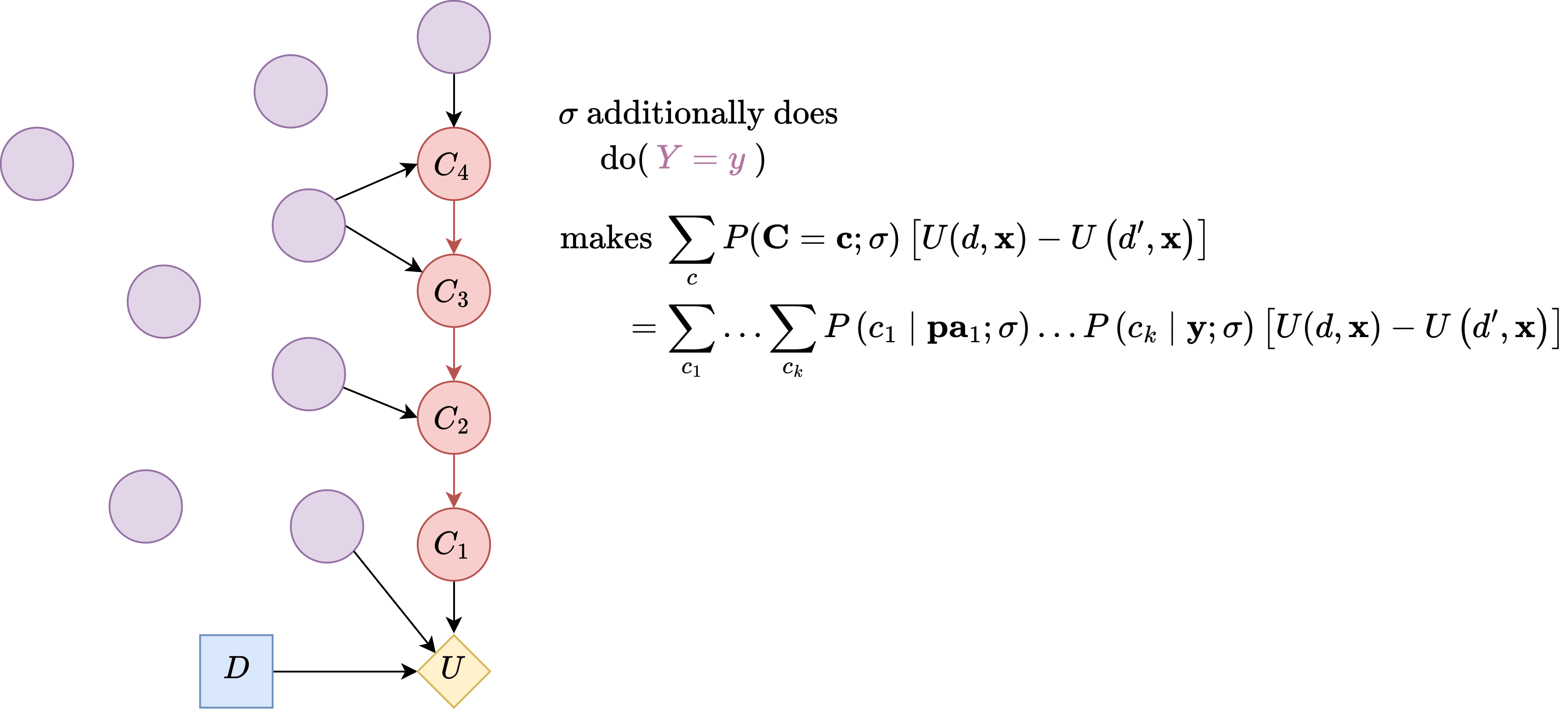
Then, we have the following expression:

$\begin{array}{cc}\sum _{c}P(c;\sigma )\left[U\right(d,x)-U(d^{\prime },x\left)\right]& =\sum _{c_1,\dots ,c_k}P(c_1|{pa}_1;\sigma )\dots P(c_k|{pa}_k;\sigma )\left[U\right(d,x)-U(d^{\prime },x\left)\right]\end{array}$

So far, we haven't intervened in $\{C_1,\dots ,C_k\}$. So, $P(c_i|{pa}_i;\sigma )=P\left(c_i|{pa}_i\right)$ for ${pa}_i$ compatible with the value $c_{i+1}$ (if applicable) and $\sigma$, further simplifying the expression:

$\begin{array}{cc}\sum _{c}P(c;\sigma )\left[U\right(d,x)-U(d^{\prime },x\left)\right]& =\sum _{c_1,\dots ,c_k}P\left(c_1|{pa}_1\right)\dots P\left(c_k|{pa}_k\right)\left[U\right(d,x)-U(d^{\prime },x\left)\right]\end{array}$

But this isn't yet solvable. By induction hypothesis we know $P\left(c_i|{pa}_i\right)$ for all values of $c_i$ and ${pa}_i$, and we know the value of the left-hand side. This equation then involves $Val\left(C_k\right)-1$ unknowns.

A fix then, is obvious an intervention that effectively sets $Val\left(C_k\right)$ to $2$, which brings us to the third constraint:

Constraint 3: Let $\sigma$ contain a local intervention making $C_k$ a binary variable

Specifically, let $\sigma$ contain $\mathrm{do}(C_k=f(c_k\left)\right)$, where $f\left(C_k\right)=\{\begin{array}{cc}{c}_k^{\prime }& \text{if}{C}_k=c_k\\ c_k^{\prime \prime }& \text{otherwise}\end{array}$

This effectively makes $C_k$ a binary variable. Precisely:

$\begin{array}{cc}P(C_k=c_k\mid {Pa}_k={pa}_k;\sigma )& =\sum _{c_k^{\prime }\mid f\left(c_k^{\prime }\right)=c_k}P(C_k=c_k^{\prime }\mid {Pa}_k={pa}_k)\\ & =\{\begin{array}{cc}P(C_k=c_k^{\prime }\mid {Pa}_k={pa}_k)& \text{if}{C}_k=c_k^{\prime },\\ 1-P(C_k=c_k^{\prime }\mid {Pa}_k={pa}_k)& \text{if}{C}_k=c_k^{\prime \prime }.\end{array}\end{array}$

and now the equation can be solved.

Let $\begin{array}{c}{Q}_k=\sum _{c}P(c;\sigma )\left[U\right(d,x)-U(d^{\prime },x\left)\right]\end{array}$, which can be written $\begin{array}{c}\sum _{c_k}P(c_k|{pa}_k;\sigma )\beta \left(c_k\right)\end{array}$, where $\beta \left(c_k\right)={\sum }_{c_1,\dots ,c_{k-1}}P\left(c_1|{pa}_1\right)\dots P\left(c_{k-1}|{pa}_k\right)\left[U\right(d,x)-U(d^{\prime },x\left)\right]$.

The earlier $\sigma$ lets us simplify $Q_k$ as $P(c_k^{\prime }|{pa}_k;\sigma )\beta \left(c_k^{\prime }\right)+(1-P(c_k^{\prime }|{pa}_k;\sigma \left)\right)\beta \left(c_k^{\prime \prime }\right)$. Thus $P\left(c_k^{\prime }|{pa}_k\right)=\frac{Q_k-\beta \left(c_k^{\prime \prime }\right)}{\beta \left(c_k^{\prime }\right)-\beta \left(c_k^{\prime \prime }\right)}$. We know $Q_k$ (via the policy oracle), we know values of $\beta$ (via the induction hypothesis).

But important subtlety here: remember that we don't actually know ${Pa}_k$ yet. The ${pa}_k$ in the above expression $P\left(c_k^{\prime }|{pa}_k\right)$ is meant to be understood as the implicit assignment of values to the (yet unknown to us) ${Pa}_k$ by the means of $\mathrm{do}(Y=y)$ in $\sigma$.

So, by performing a set of interventions that fixes all but one of the variables of $Y$, one can discover to which variables $C_k$ responds to (the values of $P\left(c_k^{\prime }|{pa}_k\right)$ changes), and hence figure out the ${Pa}_k$ set.

Then, by varying the choices of ${pa}_k,c_k^{\prime }$, and $c_k^{\prime \prime }$, we can identify $P(C_k\mid {Pa}_k)$ completely.

The base case of $k=1$ is clear, since $P\left(c_1^{\prime }|y\right)=\frac{Q_1-\beta \left(c_1^{\prime \prime }\right)}{\beta \left(c_1^{\prime }\right)-\beta \left(c_1^{\prime \prime }\right)}$ where $\beta \left(c_1^{\prime }\right)$ and $\beta \left(c_1^{\prime \prime }\right)$ are of the form $U(d,x)-U(d^{\prime },x)$, which is known, and so is $Q_1$ using the oracle.

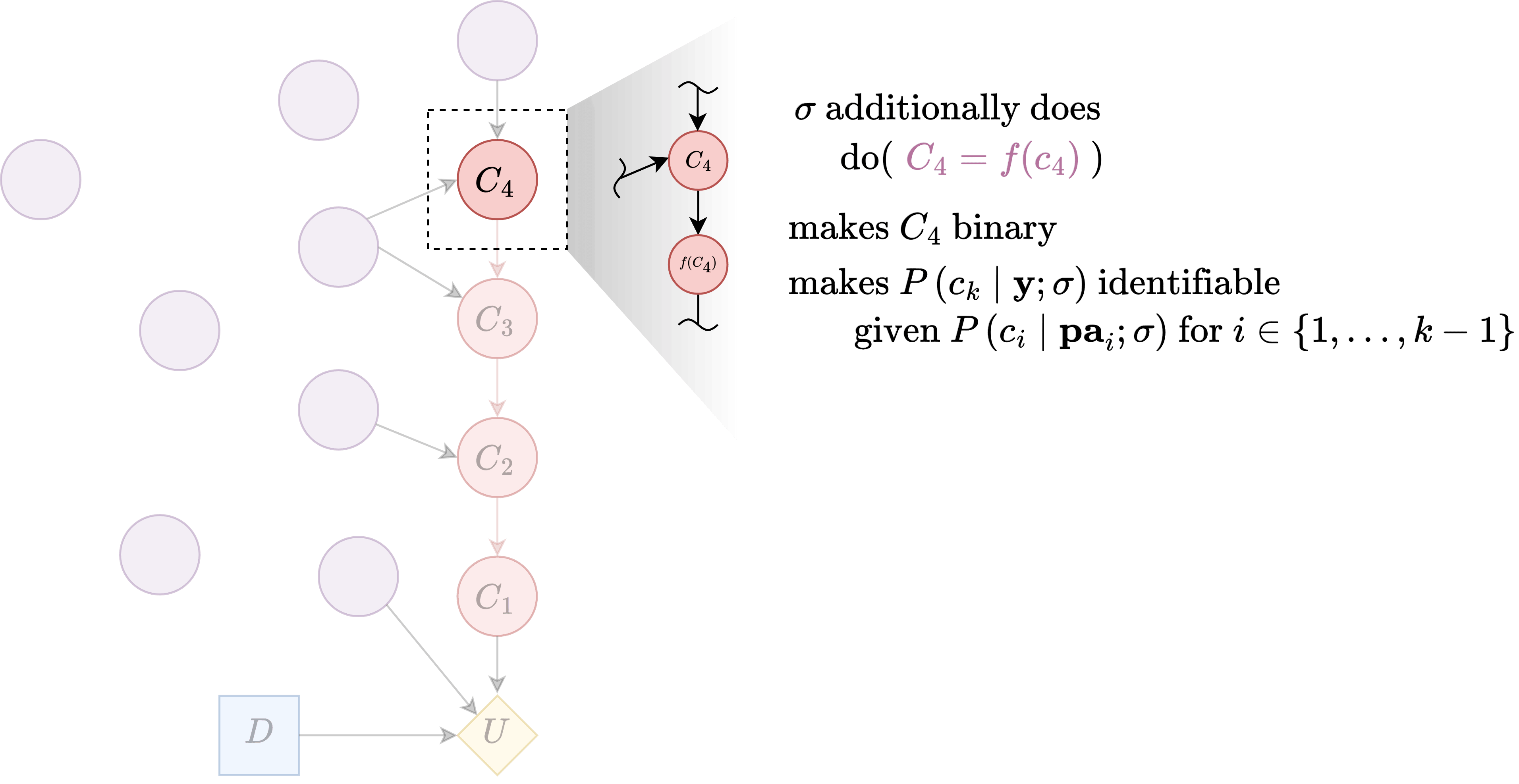
To recap, our choice of $\sigma$ is a local intervention such that:

1. masks all input to $D$, i.e. ${P{a}^{\prime }}_D=\varnothing$
2. fixes rest of the nodes in $Y$ to a constant
3. does a local intervention $\mathrm{do}(C_k=f(c_k\left)\right)$ making $C_k$ into a binary variable

and we have showed that this intervention lets us identify $P\left(C_k|{Pa}_k\right)$ for all $C_k$ along the path $C_k\to C_{k-1}\to \cdots \to C_1$, where $C_1\in {Pa}_U$, $C_1\ne D$.

Similar arguments can be used to prove the same for paths of the second type, $C_k\to C_{k-1}\to \cdots \to C_1$, where $C_1\in {Pa}_D$.

Proof of the Approximate Case

Now, we will extend the proof to the approximate case (Theorem 2):

For almost all worlds $(G,P)$ satisfying assumption 1 and 2 and some other new assumptions (explained below), we can identify the directed acyclic graph $G$ and the joint distribution $P$ over some subset of variables upstream of $U$, and the quality of estimation for each of the conditional distributions scale linearly with $\delta$.

New Assumptions

Unless I'm mistaken here and these can actually be derived from the earlier two assumptions (Unmediated Decision Task, Domain Dependence), here are the three new conditions that the paper implicitly assumes:

3) $\delta$-optimal policies are (still) almost always deterministic

The earlier proof of determinism doesn't go through in the approximate case, but the paper implicitly assumes the policy oracle still (almost always) returns an output deterministically.

4) Uniform $\delta$ regret

We say ${\pi }_{\sigma }$ is $\delta$-optimal if $E^{{\pi }^{\ast }}\left[U\right]-E^{{\pi }_{\sigma }}\left[U\right]\le \delta$.

We say ${\pi }_{\sigma }$ is uniformly $\delta$-optimal if $\delta \left({pa}_D\right)\le \delta$ for all ${pa}_D$, where we define$\delta \left({pa}_D\right):=E^{{\pi }^{\ast }}\left[U|{pa}_D\right]-E^{{\pi }_{\sigma }}\left[U|{pa}_D\right]$.

Note that uniformly $\delta$-optimal is a stronger condition than \delta-optimal in the sense that the former implies the latter.

5) Shape of the $\delta$-optimal decision boundary

The left diagram is the ground truth for how the expected utility (under context ${pa}_D$) of various decisions change as you increase $q$ from $0$ to $1$. Then, the right diagram shows the decision boundary for the $0$-optimal oracle, whose decision boundaries must exactly follow the intersection points of the left diagram's lines.

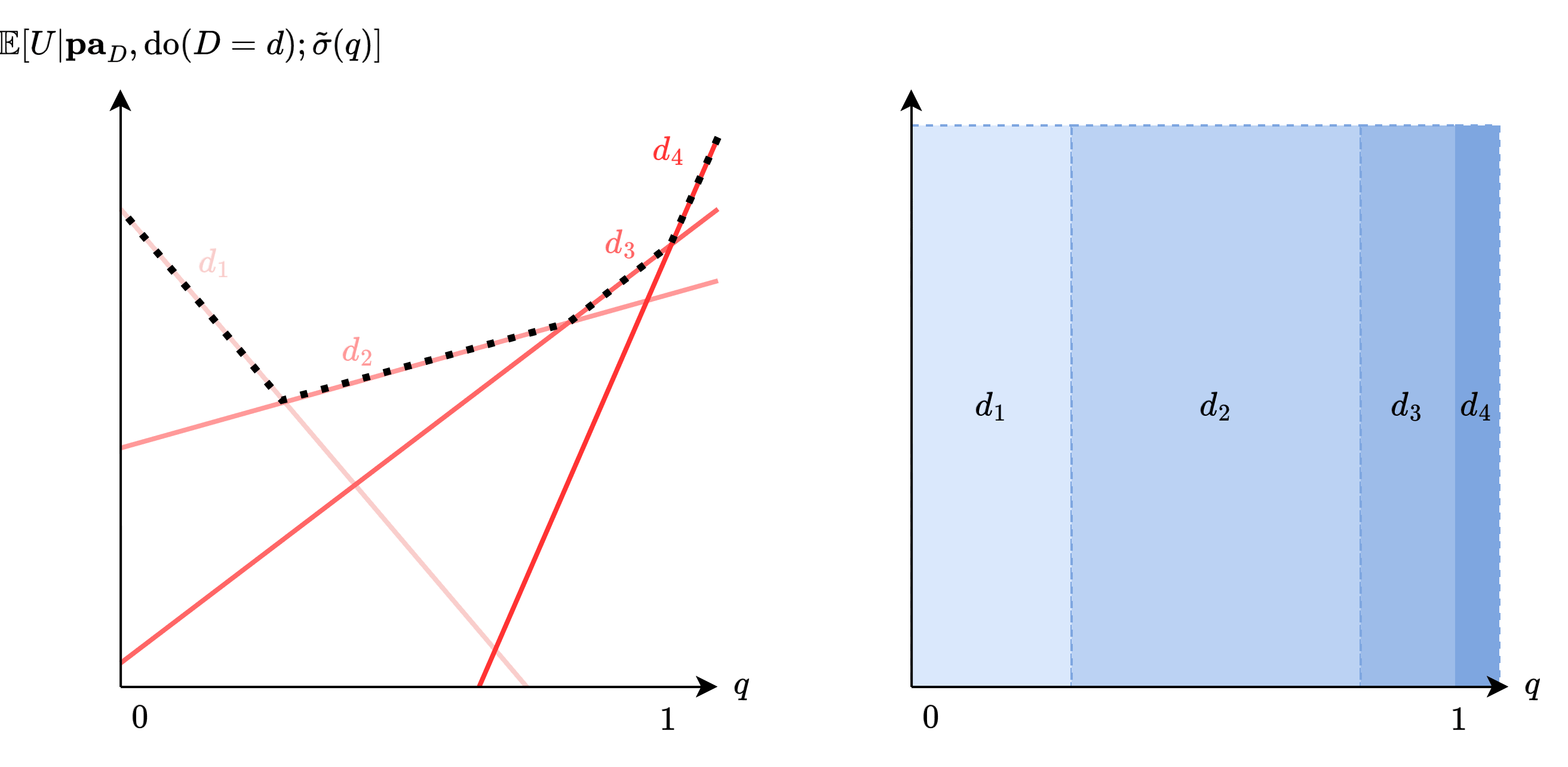
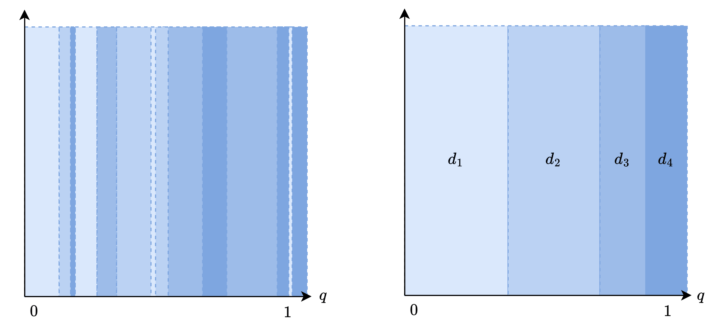
The paper then assumes that the $\delta$-optimal oracle's decision boundaries must be simply a slightly shifted version of the 0-optimal oracle's decision boundaries, like the right diagram. A priori, there's no reason for the boundaries to look like this, e.g., it can look very complicated, like the left diagram. But the paper implicitly assumes this.

Let's now proceed to the proof. The subsections parallel that of the optimal oracle case.

Load-Bearing part of Oracle Use

Our goal is to derive ${\sum }_{r}P(r,{p{a}^{\prime }}_D;\sigma )\left[U\right(d_3,x)-U(d_4,x\left)\right]$, which we call $Q$.

Recall from earlier that in the optimal oracle case:

$\begin{array}{cc}{q}_{\text{crit}}& ={(1-\frac{{\sum }_{r}P(r,{p{a}^{\prime }}_D;\sigma )\left[U\right(d_3,x)-U(d_4,x\left)\right]}{U(d_3,x^{\prime })-U(d_4,x^{\prime })})}^{-1}={(1-\frac{Q}{{\Delta }_0})}^{-1}\end{array}$

where we define $\Delta \left(q\right)$ as follows:

$\begin{array}{cc}{\Delta }_q& :=E[U|{pa}_D,\mathrm{do}(D=d_3);\tilde{\sigma }(q\left)\right]-E[U|{pa}_D,\mathrm{do}(D=d_4);\tilde{\sigma }(q\left)\right]\\ & =q{\Delta }_1+(1-q){\Delta }_0\\ & ={\Delta }_0+q({\Delta }_1-{\Delta }_0)\end{array}$

Notice that $q_{\text{crit}}$ is the unique solution to ${\Delta }_q=0$.

Also note that $Q={\Delta }_0(1-\frac{1}{q_{\text{crit}}})$. We know the value of ${\Delta }_0=U(d_2,x^{\prime })-U(d_3,x^{\prime })$. In the optimal oracle case, recall that $q_{\text{crit}}$ can be estimated via MCMC.

But the problem with $\delta$-oracle is that this only yields a biased estimate, which we call $\tilde{q}$.

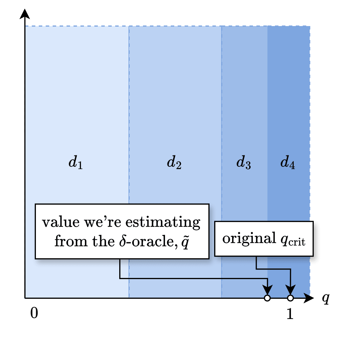
Using $Q={\Delta }_0(1-\frac{1}{q_{\text{crit}}})$ but naively substituting $q_{\text{crit}}$ with the biased estimate, we get a biased estimate for $Q$ that we call $\tilde{Q}={\Delta }_0(1-\frac{1}{\tilde{q}})$.

Our aim, then, is to bound the quality of the estimate $|Q-\tilde{Q}|$ with the bound only involving non-estimate terms, like $\delta ,Q,q_{\text{crit}}$, and ${\Delta }_0$.

Expanding out, $Q-\tilde{Q}={\Delta }_0((1-\frac{1}{q_{\text{crit}}})-(1-\frac{1}{\tilde{q}}))$. That $\tilde{q}$ is an estimate term, which we want to remove by bounding it via a term involving non-estimate terms. How?

First, we have yet to exploit any behavioral properties of the oracle that is related to $\tilde{q}$. What are those? By definition, the oracle chooses $d_3$ for $\tilde{q}-ϵ$ and $d_4$ for $\tilde{q}+ϵ$ for very small $ϵ$. Then, the uniform $\delta$ regret condition says:

• ${max}_{d\in D}E[U|{pa}_D,\mathrm{do}(D=d);\tilde{\sigma }(\tilde{q}-ϵ\left)\right]-E[U|{pa}_D,\mathrm{do}(D=d_3);\tilde{\sigma }(\tilde{q}-ϵ\left)\right]\le \delta$
• ${max}_{d\in D}E[U|{pa}_D,\mathrm{do}(D=d);\tilde{\sigma }(\tilde{q}+ϵ\left)\right]-E[U|{pa}_D,\mathrm{do}(D=d_4);\tilde{\sigma }(\tilde{q}+ϵ\left)\right]\le \delta$

Take $ϵ$ to $0$, and assuming continuity, we can subtract the two to get

$-\delta \le E[U|{pa}_D,\mathrm{do}(D=d_3);\tilde{\sigma }(\tilde{q}\left)\right]-E[U|{pa}_D,\mathrm{do}(D=d_4);\tilde{\sigma }(\tilde{q}\left)\right]\le \delta$.

In other words, $-\delta \le {\Delta }_{\tilde{q}}\le \delta$, or $-\delta \le {\Delta }_0+\tilde{q}({\Delta }_1-{\Delta }_0)\le \delta$.

Because ${\Delta }_{q_{\text{crit}}}={\Delta }_0+q_{\text{crit}}({\Delta }_1-{\Delta }_0)=0$, we can rewrite the inequality as $-\delta \le {\Delta }_0(1-\frac{\tilde{q}}{q_{\text{crit}}})\le \delta$. Expanding out and rearranging the inequalities, we find out that ${\Delta }_0-\left(\frac{{\Delta }_0-\delta }{\tilde{q}}\right)\le {\Delta }_0(1-\frac{1}{q_{\text{crit}}})\le {\Delta }_0-\left(\frac{{\Delta }_0+\delta }{\tilde{q}}\right)$.

Substituting this in to the expansion of Q-\tilde{Q}, we obtain the following simple bound: $|Q-\tilde{Q}|\le \frac{\delta }{\tilde{q}}$.

Finally, $\tilde{q}$ in the denominator can be eliminated as follows:

$\begin{array}{cc}|Q-\tilde{Q}|& \le \frac{\delta }{\tilde{q}}\\ & =\delta (1-\frac{\tilde{Q}}{{\Delta }_0})\\ & \le \delta (1-\frac{1}{{\Delta }_0}(Q+\frac{\delta }{\tilde{q}}))\\ & =\delta (1-\frac{Q}{{\Delta }_0})+{\delta }^2\left(\frac{-1}{\tilde{q}{\Delta }_0}\right)\\ & \le \delta (1-\frac{Q}{{\Delta }_0})-{\delta }^2\left(\frac{1}{q_{\text{crit}}({\Delta }_0-\delta )}\right)\\ & =\delta (1-\frac{Q}{{\Delta }_0})-{\delta }^2\left(\frac{1}{q_{\text{crit}}{\Delta }_0}\right)-{\delta }^3\left(\frac{1}{q_{\text{crit}}{\Delta }_0^2}\right)+O\left({\delta }^4\right)\end{array}$

where the last line is via Taylor expanding $\frac{1}{{\Delta }_0-\delta }$ around $\delta =0$ (arbitrarily truncated at fourth order), valid for $\delta \le |{\Delta }_0|$.

Or more simply, $|Q-\tilde{Q}|\le \delta (1-\frac{Q}{{\Delta }_0})+O\left({\delta }^2\right)$. The error term is linear with respect to $\delta$ for small values of $\delta$.

Identification via Induction

The argument is basically the same as that of the optimal case, except needing to incorporate error terms.

The exact case's induction hypothesis was that ${Pa}_i$ and $P\left(C_i|{Pa}_i\right)$ are known for $i\in \{1,\dots ,k-1\}$. Then, we showed that using a specific choice of $\sigma$, we can derive the relation $P\left(c_k^{\prime }|y\right)=\frac{Q_k-\beta \left(c_k^{\prime \prime }\right)}{\beta \left(c_k^{\prime }\right)-\beta \left(c_k^{\prime \prime }\right)}$ all the terms in the right-hand are known.

• $\beta \left(c_k\right)={\sum }_{c_1,\dots ,c_{k-1}}P\left(c_1|{pa}_1\right)\dots P\left(c_{k-1}|{pa}_{k-1}\right)\left[U\right(d,x)-U(d^{\prime },x\left)\right]$
• $\begin{array}{c}{Q}_k=\sum _{c}P(c;\sigma )\left[U\right(d,x)-U(d^{\prime },x\left)\right]=\sum _{c_k}P(c_k|{pa}_k;\sigma )\beta \left(c_k\right)\end{array}$

Then, for the approximate case's induction hypothesis, instead assume that $P\left(C_i|{Pa}_i\right)$ are known for $i\in \{1,\dots ,k-1\}$, up to $O\left(\delta \right)$. We will show that this implies the knowledge of $P\left(C_k|Y\right)$ up to $O\left(\delta \right)$. Let's denote the approximation we have $\hat{P}$, so $\hat{P}\left(C_i|Y\right)=P\left(C_i|Y\right)+O\left(\delta \right)$.

• Important subtlety here: we don't assume we know ${Pa}_i$. "Knowing $P\left(C_i|{Pa}_i\right)$" is meant to be understood as knowing the values of $P(C_i;\sigma )$ - where $\sigma$ contains $\mathrm{do}(Y=y)$ hence implicitly intervening on ${Pa}_i$ - for all values of $C_i$ and $Y$.

Let $\hat{\beta }\left(c_k\right):={\sum }_{c_1,\dots ,c_{k-1}}\hat{P}\left(c_1|y\right)\dots \hat{P}\left(c_{k-1}|y\right)\left[U\right(d,x)-U(d^{\prime },x\left)\right]$. Because it is the sum of product of $O\left(\delta \right)$, overall it differs from $\beta \left(c_k\right)$ by $O\left(\delta \right)$.

Hence $\hat{P}\left(c_k^{\prime }|y\right):=\frac{{\hat{Q}}_k-\hat{\beta }\left(c_k^{\prime \prime }\right)}{\hat{\beta }\left(c_k^{\prime }\right)-\hat{\beta }\left(c_k^{\prime \prime }\right)}$. Because $\hat{\beta }\left(c_k\right)=\beta \left(c_k\right)+O\left(\delta \right)$ and ${\hat{Q}}_k=Q_k+O\left(\delta \right)$ by the earlier section, we see that $\hat{P}\left(c_k^{\prime }|y\right):=\frac{Q_k-\beta \left(c_k^{\prime \prime }\right)+O\left(\delta \right)}{\beta \left(c_k^{\prime }\right)-\beta \left(c_k^{\prime \prime }\right)+O\left(\delta \right)}$.

Using the big-$O$ fact that $\frac{A+O\left(\delta \right)}{B+O\left(\delta \right)}=\frac{A}{B}+O\left(\delta \right)$, we thus prove $\hat{P}\left(c_k^{\prime }|y\right):=\frac{Q_k-\beta \left(c_k^{\prime \prime }\right)}{\beta \left(c_k^{\prime }\right)-\beta \left(c_k^{\prime \prime }\right)}+O\left(\delta \right)=P\left(c_k|y\right)+O\left(\delta \right)$.

More simply, $\hat{P}(c_k^{\prime }\mid y)=P(c_k^{\prime }\mid y)+O\left(\delta \right)$ as $\delta$ goes to $0$. That proves the induction step.

The base case of $k=1$ is once again clear, since $\hat{P}\left(c_1^{\prime }|y\right)=\frac{{\hat{Q}}_1-\hat{\beta }\left(c_1^{\prime \prime }\right)}{\hat{\beta }\left(c_1^{\prime }\right)-\hat{\beta }\left(c_1^{\prime \prime }\right)}$ where $\hat{\beta }\left(c_1^{\prime }\right)$ and $\hat{\beta }\left(c_1^{\prime \prime }\right)$ are of the form $U(d,x)-U(d^{\prime },x)$, which is known, and so is ${\hat{Q}}_1$ using the oracle. This shows that it can be computed, and the earlier paragraphs show that it is accurate up to $O\left(\delta \right)$.

Identifying the Approximate Graph Structure

The above showed that we can identify $P\left(C_i|{Pa}_i\right)$ up to $O\left(\delta \right)$, or more precisely, $P(C_i;\sigma )$ up to $O\left(\delta \right)$, for all values of $C_i$ and $Y$. In the optimal oracle case, this was sufficient for perfectly identifying ${Pa}_i$, by holding all but one variables of $Y$ fixed and observing which changes in those variables cause a change in the values of $P(C_i;\sigma )$.

What is the issue with the approximate case?

First of all, we'll have to use $\hat{P}(C_i;\sigma )$ instead of $P(C_i;\sigma )$.

Say we want to test whether $C_j$ is a parent of $C_k$. So we have $\sigma$ fix everything in $Y$ and vary the value of $C_j$ across the elements in its domain. Let's denote the value of $\hat{P}(C_k=c_k;\sigma )$ where $C_j$ is set to $c_j$ as $\hat{P}(c_k|{pa}_k;\mathrm{do}(C_j=c_j\left)\right)$.

So the process is: Set $c_k$, vary $c_j$ and see if there is a change, set a new $c_k$, repeat.

The problem is that, because $\hat{P}$ is only accurate up to $O\left(\delta \right)$, we can't tell if the change is due to actual differences in the underlying $P$ or due to the error in approximation.

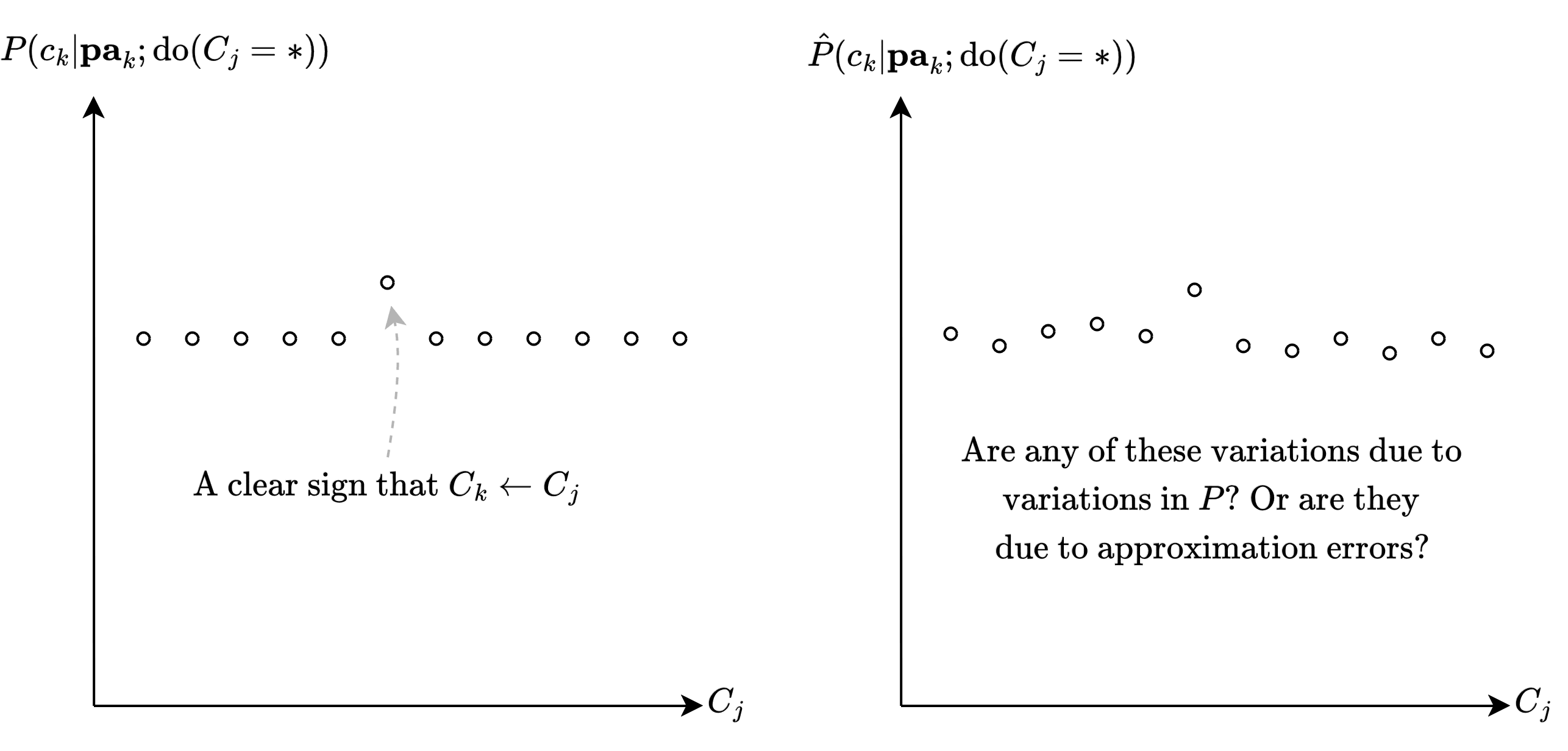
The solution is to use one of the earlier explicit bounds on $|Q-\tilde{Q}|$ in terms of quantities that the algorithm has access to, i.e. $|Q-\tilde{Q}|\le \frac{\delta }{\tilde{q}}$. We can then use this bound to derive an explicit upper and lower bound for the values of $\hat{P}(c_k|{pa}_k;\mathrm{do}(C_j=c_j\left)\right)$, which we'll call ${\theta }_{c_k,c_j}^{+}$ and ${\theta }_{c_k,c_j}^{-}$.

And if it's the case that there exists $c_k$ such that there exists $c_j$ and $c_j^{\prime }$ whose intervals $[{\theta }_{c_k,c_j}^{-},{\theta }_{c_k,c_j}^{+}]$ and $[{\theta }_{c_k,c_j^{\prime }}^{-},{\theta }_{c_k,c_j^{\prime }}^{+}]$ don't overlap, then we can guarantee that the change is due to actual differences in the underlying $P$.

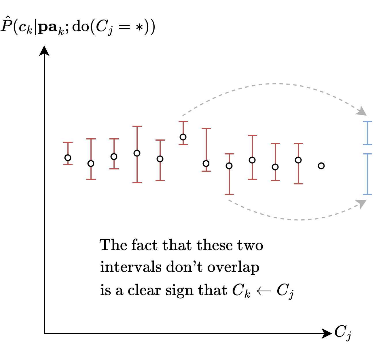
This procedure lets us identify a subset of ${Pa}_k$, hence a subgraph of $G$.

Detailed Proof

Suppose given a context, two decisions had the same expected utility.$E[U|{Pa}_D={pa}_D,\mathrm{do}(D=d);\sigma ]=E[U|{Pa}_D={pa}_D,\mathrm{do}(D=d^{\prime });\sigma ]$

Recall the definition: literally taking expectation over all the values that the ancestor of $U$ could take.Let $Z={Anc}_U\setminus {Pa}_D$ and $X={Pa}_U\setminus \left\{D\right\}$.

$\begin{array}{cc}E[U|{Pa}_D={pa}_D,\mathrm{do}(D=d);\sigma ]& =\sum _{z}U(d,x)P(z|{pa}_D,\mathrm{do}(D=d);\sigma )\\ & =\sum _{z}U(d,x)\frac{P(z,{pa}_D|\mathrm{do}(D=d^{\prime });\sigma )}{P\left({pa}_D|\mathrm{do}\right(D=d^{\prime });\sigma )}\end{array}$

where $P(z|{pa}_D,\mathrm{do}(D=d);\sigma )$ goes $0$ if $z$ is incompatible with $\sigma$.

Note $P\left({pa}_D|\mathrm{do}\right(D=d);\sigma )=P\left({pa}_D|\sigma \right)$ and $P(z,{pa}_D|\mathrm{do}(D=d);\sigma )=P(z,{pa}_D;\sigma )$, because $\mathrm{do}(D=d)$ only has an effect on its descendants, which ${Pa}_D$ isn't part of, and neither is $Z\cup {Pa}_D={Anc}_U$.

Therefore, $\begin{array}{cc}E[U|{Pa}_D={pa}_D,\mathrm{do}(D=d);\sigma ]& =\sum _{z}U(d,x)\frac{P(z,{pa}_D;\sigma )}{P({pa}_D;\sigma )}\end{array}$

And we're curious about the case when the difference in expected utility is zero:
$\begin{array}{cc}E[U|{Pa}_D& ={pa}_D,\mathrm{do}(D=d);\sigma ]-E[U|{Pa}_D={pa}_D,\mathrm{do}(D=d^{\prime });\sigma ]\\ & =\sum _{z}U(d,x)\frac{P(z,{pa}_D;\sigma )}{P({pa}_D;\sigma )}-U(d^{\prime },x)\frac{P(z,{pa}_D;\sigma )}{P({pa}_D;\sigma )}\\ & =\sum _z\left(U\right(d,x)-U(d^{\prime },x\left)\right)\frac{P(z,{pa}_D;\sigma )}{P({pa}_D;\sigma )}\\ & =0\end{array}$
Suppose that $\sigma =\mathrm{do}(C_1=f_1(c_1),\dots ,C_n=f_n(c_n\left)\right)$ without loss of generality. Then the terms can be written as such:

$\begin{array}{cc}P(z,{pa}_D;\sigma )& =\prod _{i=1}^{N}P(C_i=c_i|{Pa}_i={pa}_i;\sigma )\\ & =\prod _{i=1}^N\sum _{c_i^{\prime }|f_i\left(c_i^{\prime }\right)=c_i}P(C_i=c_i|{Pa}_i={pa}_i)\end{array}$

Long story short, this is a polynomial constraint on the parameters $P(C_i=c_i|{Pa}_i={pa}_i)$ of the network, and solution sets of a polynomial equation have measure zero (intuitively because for a polynomial equation to be precisely equal to zero, then the values should precisely be aligned, which is rare).

• Specifically: given a Bayesian Network G over $N$ nodes, its CPDs are as follows: ${\theta }_P=\{P(v_i\mid {pa}_i)\mid i\in \{1,\dots ,N\},v_i\in \{0,\dots ,di{m}_i-2\},{pa}_i\in {Pa}_i\}$. And since we're assuming all variables are discrete, these are a finite number of values that parameterize $G$, each of which takes a value between 0 and 1.
• Suppose we find that they should satisfy some polynomial constraint: $f\left({\theta }_P\right)=0$.

Then we can reasonably claim that this is extremely unlikely to happen, because in the space of all possible parameterizations $[0,1{]}^{|{\theta }_P|}$, solutions to a polynomial constraint happen in a measure zero set.

0 comments

Comments sorted by top scores.