Causal scrubbing: results on induction heads

post by LawrenceC (LawChan), Adrià Garriga-alonso (rhaps0dy), Nicholas Goldowsky-Dill (nicholas-goldowsky-dill), ryan_greenblatt, Tao Lin (tao-lin), jenny, Ansh Radhakrishnan (anshuman-radhakrishnan-1), Buck, Nate Thomas (nate-thomas) · 2022-12-03T00:59:18.327Z · LW · GW · 1 comments

Contents

  Introduction
  Methodology
    Overall approach
    Model architecture
    Identification
      Identifying induction heads
      Identifying the previous token head
    Picking out tokens at which the model is particularly likely to do induction
    Establishing a baseline
  Initial naive hypothesis
    The embeddings → value hypothesis
    The embeddings → query hypothesis
    The previous-token head → key hypothesis
    Scrubbing these all together
    Takeaways
  Refined Hypotheses
    Refined hypothesis 1
    Refined hypothesis 2
    Refined hypothesis 3
    Refined hypothesis 4
  Conclusion
  Appendices
    Model architecture and experiment details
    How we picked the subset of tokens
    Bonus refined hypothesis 5
None
1 comment

* Authors sorted alphabetically.

This is a more detailed look at our work applying causal scrubbing [LW · GW] to induction heads. The results are also summarized here [LW · GW].

Introduction

In this post, we’ll apply the causal scrubbing methodology to investigate how induction heads work in a particular 2-layer attention-only language model.^[1] While we won’t end up reaching hypotheses that are fully specific or fully human-understandable, causal scrubbing will allow us to validate claims about which components and computations of the model are important. 

We'll first identify the induction heads in our model and the distribution over which we want to explain these heads' behavior. We'll then show that an initial naive hypothesis about how these induction heads mechanistically work—similar to the one described in the Induction Heads paper (Olsson et al 2022)—only explains 35% of the loss. We’ll then go on to verify that a slightly more general, but still reasonably specific, hypothesis can explain 89% of the loss. It turns out to be the case that induction heads in this small model use information that is flowing through a variety of paths through the model – not just previous token heads and the embeddings. However, the important paths can be constrained considerably – for instance, only a small number of sequence positions are relevant and the way that attention varies in layer 0 is not that important.

As with the paren balance checker post, this post is mostly intended to be pedagogical. You can treat it as an initial foray into developing and testing a hypothesis about how induction heads work in small models. We won't describe in detail the exploratory work we did to produce various hypotheses in this document; we mostly used standard techniques (such as looking at attention patterns) and causal scrubbing itself (including looking at internal activations from the scrubbed model such as log-probabilities and attention patterns).

Methodology

Overall approach

The experiments prescribed by causal scrubbing in this post are roughly equivalent to performing resampling ablations on the parts of the rewritten model that we claim are unimportant. For each ‘actual’ datum we evaluate the loss on, we’ll always use a single ‘other’ datum for this resampling ablation.

Throughout this document we measure hypothesis quality using the percentage of the loss that is recovered under a particular hypothesis. This percentage may exceed 100% or be negative, it’s not actually a fraction. See the relevant section in the appendix post [AF · GW] for a formal definition.

Note that, in these examples, we’re not writing out formal hypotheses, as defined in our earlier post [LW · GW], because the hypotheses are fairly trivial while also being cumbersome to work with. In brief, our $I$ is identical to $G$ with all the edges we say don’t matter removed, and every node computing the identity.

Model architecture

We studied a 2-layer attention-only model with 8 heads per layer. We use L.H as a notation for attention heads where L is the zero-indexed layer number and H is the zero-indexed head number.

Further details about the model architecture (which aren’t relevant for the experiments we do) can be found in the appendix.

Identification

Identifying induction heads

Induction heads, originally described in A Mathematical Framework for Transformer Circuits (Elhage et al 2021), are attention heads which empirically attend from some token [A] back to earlier tokens [B] which follow a previous occurrence of [A]. Overall, this looks like [A][B]...[A] where the head attends back to [B] from the second [A].

Our first step was to identify induction heads. We did this by looking at the attention patterns of layer 1 heads on some text where there are opportunities for induction. These heads often either attend to the first token in a sequence, if the current token doesn’t appear earlier in the context, or look at the token following the previous occurrence of the current token.

Here are all the attention patterns of the layer 1 heads on an example sequence targeted at demonstrating induction: “Mrs. Dursley, Mr. Dursley, Dudley Dursley”

Two heads seem like possible induction heads: 1.5 and 1.6. We can make this more clear by looking more closely at their attention patterns: for instance, zooming in on the attention pattern of 1.6 we find that it attends to the sequence position corresponding to the last occurrence of  "[ley]":

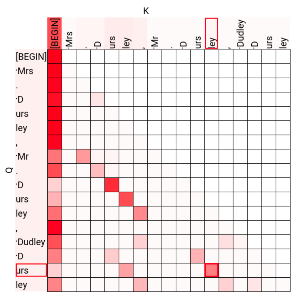
Within this, let’s specifically look at the attention from the last ‘urs’ token (highlighted in the figure above).

A closer look at the attention pattern of head 1.5 showed similar behavior.

Identifying the previous token head

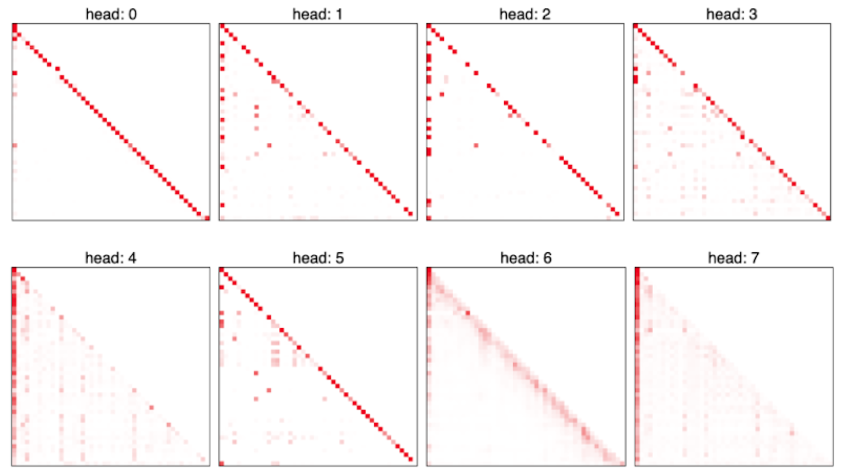
Previous token heads are heads that consistently attend to the previous token. We picked out the head that we thought was a previous token head by eyeballing the attention patterns for the layer zero heads. Here are the attention patterns for the layer zero heads on a short sequence from OpenWebText:

Here’s a plot of 0.0’s attention pattern:

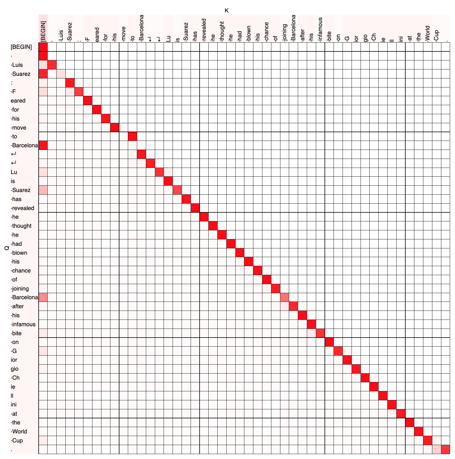
So you can see that 0.0 mostly attends to the previous token, though sometimes attends to the current token (e.g. on “ to”) and sometimes attends substantially to the [BEGIN] token (e.g. from “ Barcelona”).

Picking out tokens at which the model is particularly likely to do induction

Let's define a "next-token prediction example" to be a context (a list of tokens) and a next token; the task is to predict the next token given the context. (Normally, we train autoregressive language models on all the prefixes of a text simultaneously, for performance reasons. But equivalently, we can just think of the model as being trained on many different next-token prediction examples.)

We made a bunch of next-token prediction examples in the usual way (by taking prefixes of tokenized OWT documents), then filtered to the subset of these examples where the last token in the context was in a particular whitelist of tokens.

We chose this whitelist by following an approach which is roughly 'select tokens such that hard induction is very helpful over and above bigrams'--see the appendix [LW · GW] for further details. Code for this token filtering can be found in the appendix and the exact token list is linked. Our guess is that these results will be fairly robust to different ways of selecting the token whitelist.

So, we didn't filter based on whether induction was a useful heuristic on this particular example, or on anything about the next-token; we only filtered based on whether the last token in the context was in the whitelist.

For all the hypotheses we describe in this post, we’ll measure the performance of our scrubbed models on just this subset of next-token prediction examples. The resulting dataset is a set of sequences whose last token is somewhat selected for induction being useful. Note that evaluating hypotheses on only a subset of a dataset, as we do here, is equivalent to constructing hypotheses that make no claims on tokens other than our “inductiony” tokens, and then evaluating these weaker hypotheses on the whole dataset.

Establishing a baseline

We want to explain the performance of our two-layer attention-only model. Its performance is measured by the following computational graph:

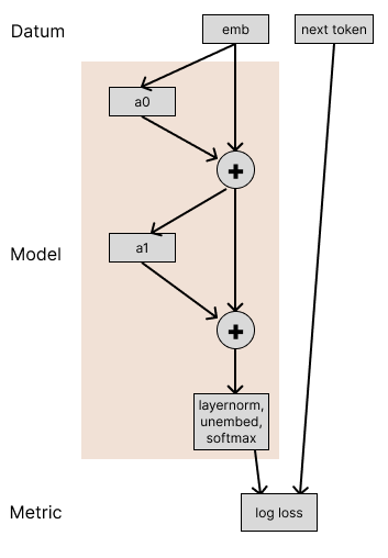
We’re taking the token embeddings (emb) and running them through the model, then calculating the log-loss of the model on the actual next token. The model is composed of two attention layers (with layernorm), which we’re writing as a0 and a1.

To start out our investigation, let’s see how much performance is damaged if we replace the induction head’s outputs with their outputs on random other sequences. To measure this, we rewrite our model to separate out the induction heads from the other layer 1 heads:

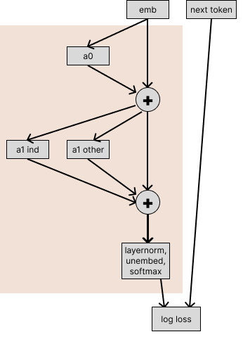
Now we consider passing in different inputs into the induction heads and the other heads.

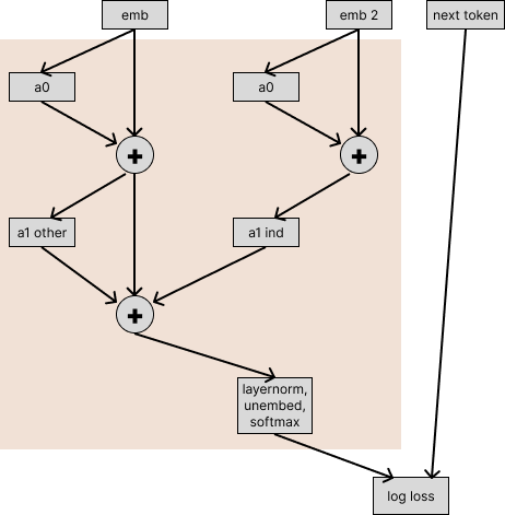
We run the model without the induction heads on the (emb, next token) pairs that correspond to sequences in our filtered next-token-prediction dataset, while running the induction heads on a different sequence (encoded as emb2).

Note that if we ran this computational graph with emb2 = emb, we’d exactly recover the performance of the original model–we’ve rewritten the model to be exactly mathematically equal, except that we’re now able to pass in inputs that are different for different paths through the model.

If the induction heads don’t contribute at all to model performance on this task, this experiment would return the same loss as the original model.

When you run the scrubbed computation, the loss is 0.213. The original loss on this dataset was 0.160, and the difference between these losses is 0.053. This confirms that the induction heads contribute significantly to the performance of the original model for this subset of tokens.

Going forward, we'll report the fraction of this 0.053 loss difference that is restored under various scrubs.

For every experiment in this post, we use the same choice of emb2 for each (emb, next token) pair. That is, every dataset example is paired with a single other sequence^[2] that we’ll patch in as required; in different experiments, the way we patch in the other sequence will be different, but it will be the same other sequence every time. We do this to reduce the variance of comparisons between experiments.

Initial naive hypothesis

This is the standard picture of induction:

• We have a sequence like “Mr. Dursley was the director of a firm called Grunnings, which made drills. He was a big, beefy man with hardly any neck, although he did have a very large mustache. Mrs. Durs”. “Dursley” is tokenized as | D|urs|ley|. And so a good prediction from the end of this sequence is “ley”. (We’ll refer to the first “urs” token as A, the first “ley” token as B, and the second “urs” token as A’.)
• There’s a previous-token head in layer 0 which copies the value at A onto B.
• The induction head at A’ attends to B because of an interaction between the token embedding at A’ and the previous-token head output at B.
• The induction head then copies the token embedding of B to its output, and therefore the model proposes B as the next token.

To test this, we need to break our induction heads into multiple pieces that can be given inputs separately. We first expand the node (highlighted in pink here):

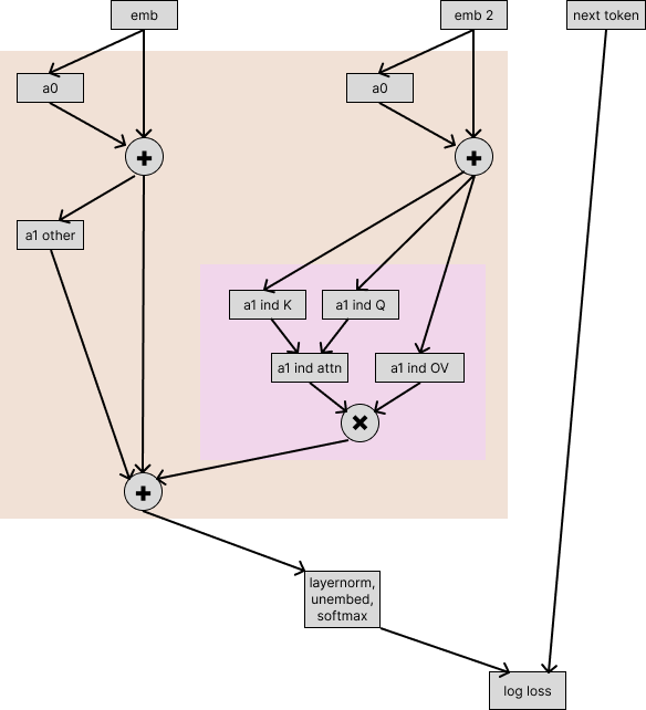
So we’ve now drawn the computation for the keys, queries, and values separately. (We’re representing the multiplications by the output matrix and the value matrix as a single “OV” node, for the same reasons as described in the “Attention Heads are Independent and Additive” section of A Mathematical Framework for Transformer Circuits.)

Our hypothesis here involves claims about how the queries, keys, and values are formed:

• values for the induction head are produced only from the token embeddings via the residual stream with no dependence on a0
• queries are also produced only from the token embeddings
• keys are produced only by the previous-token head

Before we test them together, let’s test them separately.

The embeddings → value hypothesis

The hypothesis claims that the values for the induction head are produced only from the token embeddings via the residual stream, with no dependence on a0. So, it it shouldn’t affect model behavior if we rewrite the computation such that the a1 induction OV path is given the a0 output from emb2, and so it only gets the information in emb via the residual connection around a0:

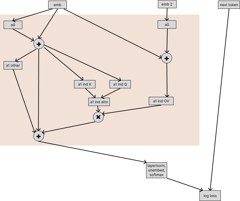
When we do this scrub, the measured loss is 90% of the way from the baseline ablated model (where we ran the induction heads on emb2) to the original unablated model. So the part of the hypothesis where we said only the token embeddings matter for the value path of the induction heads is somewhat incorrect.

The embeddings → query hypothesis

We can similarly try testing the “the queries for induction heads are produced only from the token embeddings” hypothesis, with the following experiment:

The fraction of the loss restored in this experiment is 51%, which suggests that this part of the hypothesis was substantially less correct than the part about how the induction head values are produced.

The previous-token head → key hypothesis

Finally, we want to test the final claim in our hypothesis; that the key used by the induction head is produced only by the previous-token head.

To do this, we first rewrite our computational graph so that the induction key path takes the previous-token head separately from the other layer zero heads.

This experiment here aims to evaluate the claim that the only input to the induction heads that matters for the keys is the input from the previous-token head.

However, this experiment wouldn’t test that the previous-token head is actually a previous token head. Rather, it just tests that this particular head is the one relied on by the induction heads.

We can make a strong version of this previous token head claim via two sub-claims:

• The attention pattern is unimportant (by which we mean that the relationship between the attention pattern and the OV is unimportant, as discussed in this section of our earlier post)
• All that matters for the OV is the previous sequence position

We’ll implement these claims by rewriting the model to separate out the parts which we claim are unimportant and then scrubbing these parts. Specifically, we’re claiming that this head always operates on the previous token through its OV (so we connect that to “emb”); and its attention pattern doesn’t depend on the current sentence (so we connect that to “emb2”). We also connect the OV for tokens that are not the previous one to “emb2”.

The resulting computation for the previous-token head is as follows:

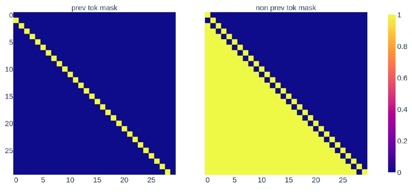
So we’ve run the OV circuit on both emb and emb2, and then we multiply each of these by a mask so that we only use the OV result from emb for the previous token. Prev mask is a matrix that is all zeros except for the row below the diagonal (corresponding to attention to the previous token). Non prev mask is the difference between prev mask and the lower triangular mask that we normally use to enforce that attention only looks at previous sequence positions.

And so, our overall experiment is as follows, where the nodes of the model corresponding to the previous token head are shown in pink:

This fraction of the loss restored by this experiment is 79%.

Scrubbing these all together

Next we want to scrub all these paths (i.e. do all these interventions) simultaneously.

The fraction of the loss that this restores is 35%.

Takeaways

Using causal scrubbing, we’ve found that our initial naive hypothesis is quite incorrect for these induction heads.

To recap the results, the fractions of loss restored are:

• Scrubbing all of the input to Q except the embeddings: 51%.
• Scrubbing all of the input to K, except the previous token part of the previous-token head: 79%
• Scrubbing all of the input to V except the embeddings: 90%
• Doing all of these at once: 35%

These numbers weren’t very surprising to us. When we described this experiment to some of the authors of the induction heads paper, we asked them to guess the proportion of loss that this would recover, and their answers were also roughly in the right ballpark.

Refined Hypotheses

Refined hypothesis 1

How might our previous hypothesis be missing important considerations? Or, to put it differently, what important information are we scrubbing away?

One possibility is that it’s common for attention heads to attend substantially to the current sequence position (you’ll see this if you look at the attention patterns included in the “Identification” section). This attention results in the token’s representation being transformed in a predictable way. And so, when the induction heads are learning to e.g. copy a token value, they’ll probably set up their V matrix to take into account the average attention-to-current-token of the layer zero heads.

We would like to express the hypothesis that the induction head interacts with all the layer zero heads, but through their average attention-to-current-token. That is, we hypothesize that the induction head’s behavior isn’t importantly relying on the ways that a0 heads vary their attention depending on context; it’s just relying on the effect of the a0 head OV pathway, ignoring correlation with the a0 attention pattern.

Similarly, there might be attention heads other than the previous token head which, on average, attend substantially to the previous token; the previous hypothesis also neglects this, but we’d like to represent it.

Here’s the complete experiment we run. Things to note:

• We’ve drawn the “emb” and “emb2” nodes multiple times. This is just for ease of drawing–we’ll always use the same value the two places we drew an emb node.
• The main point of this experiment is that the layer zero attention patterns used by the induction heads always come from emb2, so the induction heads can’t be relying on any statistical relationship between the layer zero attention pattern and the correct next token.

Running parts of this individually (that is, just scrubbing one of Q, K, or V in the induction heads, while giving the others their value on emb) and all together (which is what is pictured) yields the following amounts of loss recovered:

Q: 76%
K: 86%
V: 97%
All: 62%

So, we've captured V quite well with this addition, but we haven’t yet captured much of what’s happening with K and Q.

Refined hypothesis 2

One theory for what could be going wrong with Q and K is that we need to take into account other sequence positions. Specifically, maybe there's some gating where K only inducts on certain 'B' tokens in AB...A, and maybe the induction heads fire harder on patterns of the form XAB...XA, where there are two matching tokens (for example, in the earlier Dursley example, note that the two previous tokens | D| and |urs| both matched.). This is certainly not a novel idea—prior work has mentioned fuzzy matching on multiple tokens.

So, we'll considerably expand our hypothesis by including 'just the last 3 tokens' for K and Q (instead of just previous and just current). (By last three, we mean current, previous, and previous to previous.)

It’s getting unwieldy to put all this in the same diagram, so we’ll separately draw how to scrub K, Q, and V. The OV activations are produced using the current token mask, and the Q and K are produced using the “last 3 mask”. Both use the direct path from emb rather than emb2.

Given these, we can do the experiments for this hypothesis by substituting in those scrubbed activations as desired:

And the numbers are:

Q: 87%
K: 91%
V: 97% (same as previous)
All: 76%

This improved things considerably, but we're still missing quite a bit. (We tested using different subsets of the relative sequence positions for Q and K; using the last three for both was the minimal subset which captures nearly all of the effect.)

Refined hypothesis 3

If you investigate what heads in layer 0 do, it turns out that there are some heads which often almost entirely attend to occurrences of the current token, even when it occurred at earlier sequence positions.

The below figure shows the attention pattern of 0.2 for the query at the last ' Democratic' token:

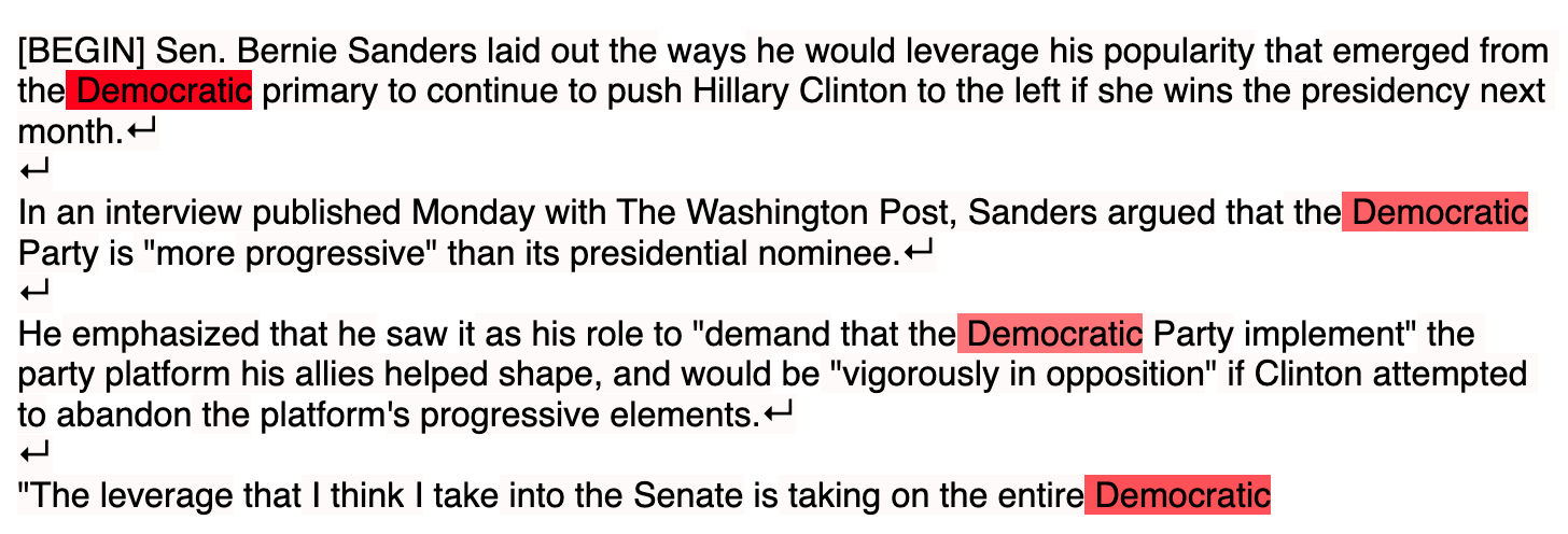
So you can see that 0.2 attended to all the copies of “ Democratic”.

Because this is a layer zero head, the input to the attention head is just the token embedding, and so attending to other copies of the same token leads to the same output as the head would have had if it had just attended to the current token. But it means that on any particular sequence, this head’s attention pattern is quite different from its attention pattern averaged over sequences. Here is that head’s attention pattern at that sequence position, averaged over a large number of sequences:

On average, this head attends mostly to the current token, a bit to the [BEGIN] token, and then diffusely across the whole sequence. This is the average attention pattern because tokens that match the current token are similarly likely to be anywhere in the context.

These heads have this kind of attend-to-tokens-that-are-the-same-as-the-current-token behavior for most of the tokens in the subset of tokens that we picked (as described in “Picking out inductiony tokens”). This is problematic for our strategy where we scrub the attention probabilities because the expected attention probability on tokens matching the current token might be 0.3, even though the model always only attends to tokens matching the current token.

There are two-layer 0 heads which most clearly have this behavior, 0.2 and 0.5, as well as 0.1, which somewhat has this behavior.

(These heads don't just do this. For instance, in the attention pattern displayed above, 0.2 also attends to ' Democratic' and ' Party' from the ' GOP' token. We hypothesize this is related to 'soft induction'^[3], though it probably also has other purposes – for instance directly making predictions from bigrams and usages in other layer 1 heads.)

In addition to this issue with the self-attending heads, the previous token head also sometimes deviates from attending to the previous token, and this causes additional noise when we try to approximate it by its expectation. So, let’s try the experiment where we run the previous token head and these self-attending heads with no scrubbing or masking.

So we’re computing the queries and keys for the induction heads as follows:

And then we use these for the queries and keys for the induction heads. We use the same values for the induction heads as in the last experiment. Our experiment graph is the same as the last experiment, except that we’ve produced Q and K for the induction heads in this new way.

Now we get:

Q: 98%
K: 97%
V: 97% (same as previous)
All: 91%

We’re happy with recovering this much of the loss, but we aren’t happy with the specificity of our hypothesis (in the sense that a more specific hypothesis makes more mechanistic claims and permits more extreme intervention experiments). Next, we’ll try to find a hypothesis that is more specific while recovering a similar amount of the loss.

Refined hypothesis 4

So we’ve observed that the self-attending heads in layer zero are mostly just attending to copies of the same token. This means that even though these heads don’t have an attention pattern that looks like the identity matrix, they should behave very similarly to how they’d behave if their attention pattern was the identity matrix. If we can take that into account, we should be able to capture more of how the queries are formed.

To test that, we rewrite the self-attending heads (0.1, 0.2, 0.5) using the $a=b+(a-b)$ identity, where “identity attention” means the identity matrix attention pattern:

This is equal to calculating 0.1, 0.2, and 0.5 the normal way, but it permits us to check the claim “The outputs of 0.1, 0.2, and 0.5 don’t importantly differ from what they’d be if they always attended to the current token”, by using just the left hand side from the real input and calculating the “error term” using the other input.

Let’s call this “0.1, 0.2, 0.5 with residual rewrite”.

So now we have a new way of calculating the queries for the induction heads:

Aside from the queries for the induction heads, we run the same experiment as refined hypothesis 2.

And this yields:

Q: 97%
K: 91% (same as refined hypothesis 2)
V: 97% (same as refined hypothesis 2)
All: 86%

We've now retained a decent fraction of the loss while simultaneously testing a reasonably specific hypothesis for what is going on in layer 0.

Conclusion

In this post, we used causal scrubbing to test a naive hypothesis about induction heads, and found that it was incorrect. We then iteratively refined four hypotheses using the scrubbed expectation as a guide. Hopefully, this will serve as a useful example of how causal scrubbing works in simple settings.

Key takeaways:

• We were able to use causal scrubbing to narrow down what model computations are importantly involved in induction.
• In practice, induction heads in small models take into account information from a variety of sources to determine where to attend.

Appendices

Model architecture and experiment details

• The model uses the shortformer positional encodings (which means that the positional embeddings are added into the Q and K values before every attention pattern is computed, but are not provided to the V)
• The model has layer norms before the attention layers
• The model was trained on the openwebtext dataset
• Its hidden dimension is 256
• We ran causal scrubbing on validation data from openwebtext with sequence length 300

How we picked the subset of tokens

Choose beta and threshold. Then for all sequential pairs of tokens, AB, in the corpus we compute:

• The log loss of the bigram probabilities $P_{\text{bigram}}$ (via the full bigram matrix).
• The log loss of the beta-level induction heuristic probabilities $P_{\beta \text{-induction}}$. Intuitively, this heuristic upweights the probability of B based on how frequently A has been followed by B in the context. We compute these probabilities as:
  • Find all prior occurrences of A in the same input datum
  • Count the number of these prior occurrences which are followed by B. Call this the matching count $m$. Let the remaining occurrences be the not matching count, $n$.
  • Starting from the bigram statistics, we add $\beta \ast m$ to the logit of B and $\beta \ast n$ to the not-B logit. That is:$P_{\beta \text{-induction}}\left(B|A\right)=\sigma \left(\log P_{\text{bigram}}\right(B|A)+\beta \cdot m-\log P_{\text{bigram}}(\neg B|A\left)\right)-\beta \cdot n)$
  • Then, we compute the log loss of these probabilities.
• Finally, we compute the average log loss from the A for each of these two heuristics. If the bigram loss is larger than the induction heuristic loss by at least some small threshold for a given A token, we include that token.

(We can also run the same experiments while evaluating the loss on all tokens; this decreases the loss recovered relative to evaluating on just this subset.)

Bonus refined hypothesis 5

Our previous hypothesis improved the Q pathway considerably, but we’re missing quite a bit of loss due to scrubbing the attention pattern of the previous token head for K. This is due to cases where the previous token head deviates from attending to the previous token. If we sample an alternative sequence which fails to attend to the previous token at some important location, this degrades the induction loss. We’ll propose a simple hypothesis which partially addresses this issue.

Consider the following passage of text:

[BEGIN] I discovered Chemis artwork a few weeks ago in Antwerp (Belgium) I’ve been fascinated by the poetry of his murals and also by his fantastic technique. He kindly accepted to answer a few questions for StreetArt360. Here’s his interview.\n\nHello Dmitrij, great to meet you.

We’ll look at the attention pattern for the previous token head as weighted lines from q tokens to k tokens.

For instance, here’s the start of the sequence:

Some utf-8 characters consist of multiple bytes and the bytes are tokenized into different tokens. In this case, those black diamonds are from an apostrophe being tokenized into 2 tokens.

Note that the previous token head exhibits quite different behavior on  I’ve (where the apostrophe is tokenized into those 2 black diamonds). Specifically, ve skips over the apostrophe to attend to  I. The token  been also does this to some extent.

Another common case where the previous token head deviates is on punctuation. Specifically, on periods it will often attend to the current token more than typical.

While there are a variety of different contexts in which the previous token head importantly varies its attention, we’ll just try to explain a bit of this behavior. We’ll do this by identifying a bunch of cases where the head has atypical behavior.

It turns out that the model special cases a variety of different quote characters. We’ll specifically reference ', “,  “, and ”.

It’s a bit hard to read this, so here’s a zoomed in version with a font that makes the different characters more obvious.

These quote characters each consist of two tokens and the head has atypical behavior if any of those tokens is the previous one.

It turns out the model also sometimes has atypical behavior if the previous token is the  a or  an token:

And, it has atypical behavior if the current token is . or  to.

Overall, here is simple classifier for whether or not a given token is atypical:

• Is the previous token one of the bytes from any of: ’,  “,   “, and ”? If so, atypical.
• Is the previous token one of  a or  an? If so, atypical.
• Is the current token one of . or  to? If so, atypical.
• Otherwise, typical.

And we’ll propose that it only matters whether or not the attention from the current location should be ‘typical’ or ‘atypical’. Then, we can test this hypothesis with causal scrubbing by sampling the attention pattern from the current location from a different sequence which has the same ‘typicality’ at that location.

This hypothesis is clearly somewhat wrong – it doesn’t only matter whether or not the current token is ‘typical’! For instance, the current token being . or  to results in attending to the previous token while the previous token being  a results in attending two back. Beyond this issue, we’ve failed to handle a bunch of cases where the model has different behavior. This hypothesis would be easy to improve, but we’ll keep it as is for simplicity.

We’ll apply this augmented hypothesis for the previous token head to just the K pathway. This yields:

Q: 97% (same as refined hypothesis 4)
K: 94%
V: 97% (same as refined hypothesis 2)
All: 89%

So compared to refined hypothesis 4, this improved the loss recovered by 3% for both K individually (94 -> 97%) and everything together (86->89%). This brings us considerably closer to the overall loss from hypothesis 3 which was 91%.

1. ^{^}

    These heads are probably doing some things in addition to induction; we’ll nevertheless refer to them as induction heads for simplicity and consistency with earlier work.

2. ^{^}

    Note that we opt to use a single input rather than many [LW · GW].

3. ^{^}

    This is where seeing AB updates you towards thinking that tokens similar to A are likely to be followed by tokens like B.

1 comments

Comments sorted by top scores.