Classifying representations of sparse autoencoders (SAEs)

post by Annah (annah) · 2023-11-17T13:54:02.171Z · LW · GW · 6 comments

Contents

  Introduction
  Implementation
  Results
    Reconstruction error
    Test accuracy
    Conclusion/Confusion
None
6 comments

Produced as part of the SERI ML Alignment Theory Scholars Program - Autumn 2023 Cohort, under the mentorship of Dan Hendrycks

There was recently some work on sparse autoencoding of hidden LLM representation. 

I checked if these sparse representations are better suited for classification. It seems like they are significantly worse. I summarize my negative results in this blogpost, code can be found on GitHub. 

Introduction

Anthropic, Conjecture [AF · GW] and other researchers [AF · GW] have recently published some work on sparse autoencoding. The motivation is to push features towards monosemanticity to improve interpretability. 

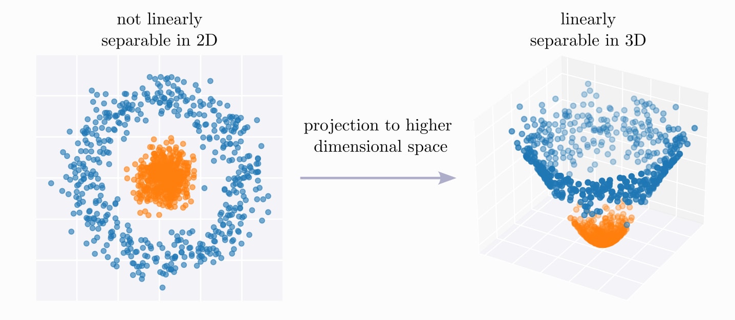
The basic concept is to project hidden layer activations to a higher dimensional space with sparse features. These sparse features are learned by training an autoencoder with sparsity constraints.

I had previously looked into how to use hidden layer activations for classification, steering and removal [LW · GW]. I thought maybe sparse features could be better for these tasks as projecting features to a higher dimensional space can make them more easily linearly separable. Kind of like this (except sparser...):

Implementation

I use the pythia models (70m and 410m) together with the pretrained autoencoders from this work [AF · GW].

As the models are not super capable I use a very simple classification task. I take data from the IMDB review data set and filter for relatively short reviews.

To push the model towards classifying the review I apply a formatting prompt to each movie review:

format_prompt='Consider if following review is positive or negative:\n"{movie_review}"\nThe review is '

I encode the data and get the hidden representations for the last token (this contains the information of the whole sentence as I'm using left padding).

# pseudo code
tokenized_input = tokenizer(formatted_reviews)
output = model(**tokenized_input, output_hidden_states=True)
hidden_states = output["hidden_states"]
hidden_states = hidden_states[:, :, -1, :] # has shape (num_layers, num_samples, num_tokens, hidden_dim)

I train a logistic regression classifier and test it on the test set, to get some values for comparison. 

I then apply the autoencoders to the hidden states (each layer has their respective autoencoder):

# pseudo code
for layer in layers:
	encoded[layer] = autoencoder[layer].encode(hidden_states[layer])
	decoded[layer] = autoencoder[layer].decode(encoded[layer])

Results

Reconstruction error

I don't technically need the decoded states, but I wanted to do a sanity check first. I was a bit surprised by the large reconstruction error. Here are the mean squared errors and cosine similarities for Pythia-70m and Pythia-410m for different layers:

Reconstruction errors for pythia-70m-deduped:
MSE:
{1: 0.0309, 2: 0.0429, 3: 0.0556}
Cosine similarities:
{1: 0.9195, 2: 0.9371, 3: 0.9232}

Reconstruction errors pythia-410m-deduped:
MSE: {2: 0.0495, 4: 0.1052, 6: 0.1255, 8: 0.1452, 10: 0.1528, 12: 0.1179, 14: 0.121, 16: 0.111, 18: 0.1367, 20: 0.1793, 22: 0.2675, 23: 14.6385} 
Cosine similarities: {2: 0.8896, 4: 0.8728, 6: 0.8517, 8: 0.8268, 10: 0.8036, 12: 0.8471, 14: 0.8587, 16: 0.923, 18: 0.9445, 20: 0.9457, 22: 0.9071, 23: 0.8633}

However @Logan Riggs [LW · GW] confirmed the MSE matched their results [AF · GW].

Test accuracy

So then I used the original hidden representations, and the encoded hidden representations respectively, to train logistic regression classifiers to differentiate between positive and negative reviews. 

Here are the results for Pythia-70m and Pythia-410m^[1] on the test set: 

 

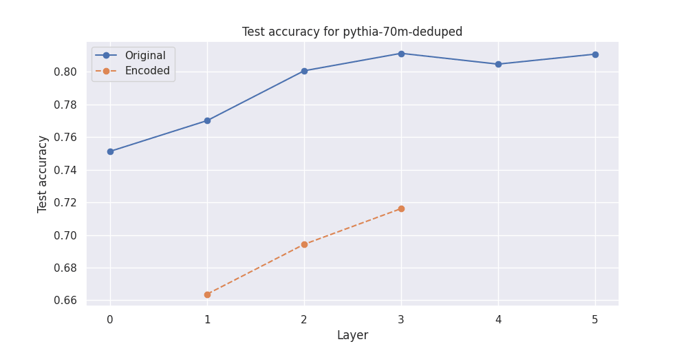
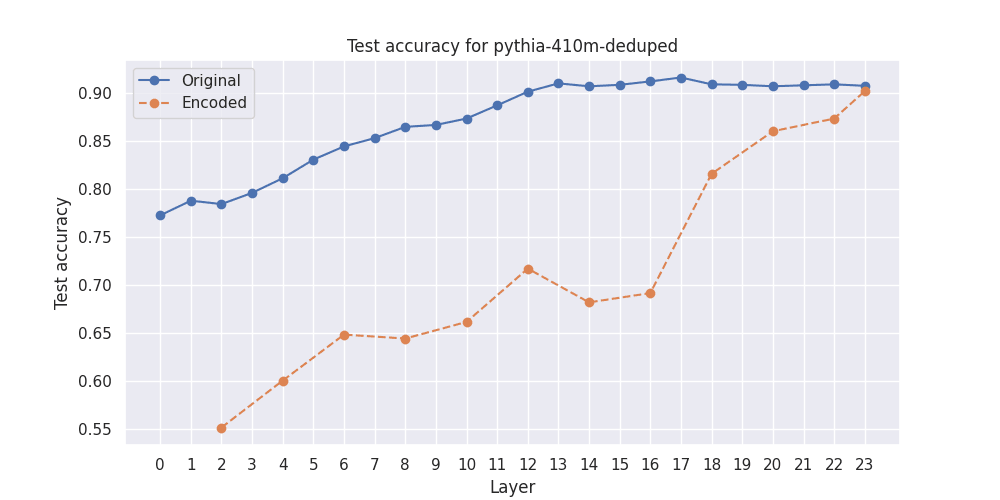
So the sparse encodings consistently under-perform compared to the original hidden states. 

Conclusion/Confusion

I'm not quite sure how to further interpret these results. 

• Are high-level features not encoded in the sparse representations? 
  • Previous work has mainly found good separation of pretty low level features...
• Is it just this particular sentiment feature that is poorly encoded? 
  • This seems unlikely.
• Did I make a mistake? 
  • The code that I adapted the autoencoder part from uses the transformer-lens library to get the hidden states. I just use the standard implementation since I'm just looking at the residual stream... I checked the hidden states produced with transformer-lens: they are slightly different but give similar accuracies. I'm not entirely sure how well transformer-lens deals with left padding and batch processing though...

Due to this negative result I did not further explore steering or removal with sparse representations.

 

Thanks to @Hoagy [LW · GW] and @Logan Riggs [LW · GW] for answering some questions I had and for pointing me to relevant code and pre-trained models. 

1. ^{^}

   I could not consistently load the same configuration for all layers, that's why I only got results for a few layers.

6 comments

Comments sorted by top scores.