DaemonicSigil's Shortform
post by DaemonicSigil · 2023-08-20T22:58:57.385Z · LW · GW · 12 commentsContents
12 comments
12 comments
Comments sorted by top scores.
comment by DaemonicSigil · 2024-06-01T06:54:48.474Z · LW(p) · GW(p)
If you're working with multidimensional tensors (eg. in numpy or pytorch), a helpful pattern is often to use pattern matching to get the sizes of various dimensions. Like this: batch, chan, w, h = x.shape. And sometimes you already know some of these dimensions, and want to assert that they have the correct values. Here is a convenient way to do that. Define the following class and single instance of it:
class _MustBe:
  """ class for asserting that a dimension must have a certain value.
      the class itself is private, one should import a particular object,
      "must_be" in order to use the functionality. example code:
      `batch, chan, must_be[32], must_be[32] = image.shape` """
  def __setitem__(self, key, value):
    assert key == value, "must_be[%d] does not match dimension %d" % (key, value)
must_be = _MustBe()
This hack overrides index assignment and replaces it with an assertion. To use, import must_be from the file where you defined it. Now you can do stuff like this:
batch, must_be[3] = v.shape
must_be[batch], l, n = A.shape
must_be[batch], must_be[n], m = B.shape
...
Linkpost for: https://pbement.com/posts/must_be.html
comment by DaemonicSigil · 2024-06-15T02:27:01.649Z · LW(p) · GW(p)
People here might find this post interesting: https://yellow-apartment-148.notion.site/AI-Search-The-Bitter-er-Lesson-44c11acd27294f4495c3de778cd09c8d
The author argues that search algorithms will play a much larger role in AI in the future than they do today.
comment by DaemonicSigil · 2024-02-19T04:14:16.969Z · LW(p) · GW(p)
Perturbation Theory in Machine Learning
Linkpost for: https://pbement.com/posts/perturbation_theory.html
In quantum mechanics there is this idea of perturbation theory, where a Hamiltonian is perturbed by some change to become . As long as the perturbation is small, we can use the technique of perturbation theory to find out facts about the perturbed Hamiltonian, like what its eigenvalues should be.
An interesting question is if we can also do perturbation theory in machine learning. Suppose I am training a GAN, a diffuser, or some other machine learning technique that matches an empirical distribution. We'll use a statistical physics setup to say that the empirical distribution is given by:
Note that we may or may not have an explicit formula for . The distribution of the perturbed Hamiltonian is given by:
The loss function of the network will look something like:
Where are the network's parameters, and is the per-sample loss function which will depend on what kind of model we're training. Now suppose we'd like to perturb the Hamiltonian. We'll assume that we have an explicit formula for . Then the loss can be easily modified as follows:
If the perturbation is too large, then the exponential causes the loss to be dominated by a few outliers, which is bad. But if the perturbation isn't too large, then we can perturb the empirical distribution by a small amount in a desired direction.
One other thing to consider is that the exponential will generally increase variance in the magnitude of the gradient. To partially deal with this, we can define an adjusted batch size as:
Then by varying the actual number of samples we put into a batch, we can try to maintain a more or less constant adjusted batch size. One way to do this is to define an error variable, err = 0. At each step, we add a constant B_avg to the error. Then we add samples to the batch until adding one more sample would cause the adjusted batch size to exceed err. Subtract the adjusted batch size from err, train on the batch, and repeat. The error carries over from one step to the next, and so the adjusted batch sizes should average to B_avg.
↑ comment by Gunnar_Zarncke · 2024-02-19T08:45:11.692Z · LW(p) · GW(p)
What is the difference between a perturbation and the difference from a gradient in SGD? Both seem to do the same thing. I'm just pattern-matching and don't know too much of either.
Replies from: DaemonicSigil↑ comment by DaemonicSigil · 2024-02-19T21:04:56.235Z · LW(p) · GW(p)
In this context, we're imitating some probability distribution, and the perturbation means we're slightly adjusting the probabilities, making some of them higher and some of them lower. The adjustment is small in a multiplicative sense not an additive sense, hence the use of exponentials. Just as a silly example, maybe I'm training on MNIST digits, but I want the 2's to make up 30% of the distribution rather than just 10%. The math described above would let me train a GAN that generates 2's 30% of the time.
I'm not sure what is meant by "the difference from a gradient in SGD", so I'd need more information to say whether it is different from a perturbation or not. But probably it's different: perturbations in the above sense are perturbations in the probability distribution over the training data.
Replies from: Gunnar_Zarncke↑ comment by Gunnar_Zarncke · 2024-02-19T23:31:09.042Z · LW(p) · GW(p)
Thanks. Your ΔH looked like ∇Q from gradient descent, but you don't intend to take derivatives, nor maximize x, so I was mistaken.
comment by DaemonicSigil · 2023-08-20T22:58:57.501Z · LW(p) · GW(p)
On George Hotz's doomcorp idea:
George Hotz has an idea which goes like so (this is a paraphrase): If you think an AGI could end the world, tell me how. I'll make it easy for you. We're going to start a company called Doomcorp. The goal of the company is to end the world using AGI. We'll assume that this company has top-notch AI development capabilities. How do you run Doomcorp in such a way that the world has ended 20 years later?
George accepts that Doomcorp can build an AGI much more capable and much more agent-like than GPT-4. He also accepts that this AGI can be put in charge of Doomcorp (or put itself in charge) and run Doomcorp. The main question is: how do you go from there to the end of the world?
Here's a fun answer: Doomcorp becomes a military robot company. A big part of the difficulty with robots in the physical world is the software. (AI could also help with hardware design, of course.) Doomcorp provides the robots, complete with software that allows them to act in the physical world with at least a basic amount of intelligence. Countries that don't want to be completely unable to defend themselves in combat are going to have to buy the robots to be competitive. How does this lead to the eventual end of the world? Backdoors in the bot software/hardware. It just takes a signal from the AI to turn the bots into killing machines perfectly willing to go and kill all humans.
Predicted geohot response: I strongly expect a multipolar takeoff where no one AI is stronger than any of the others. In such a world, there will be many different military robot companies, and different countries will buy from different suppliers. Even if the robots from one supplier did the treacherous turn thing, the other robots would be strong enough to fight them off.
Challenge: Can you see a way for Doomcorp to avoid this difficulty? Try and solve it yourself before looking at the spoiler.
The company building a product isn't the only party that can get a backdoor into that product. Paid agents that are employees of the company can do it, hacking into the company's systems is another method, as are supply chain attacks. Speaking of this last issue, consider this. An ideal outcome from the perspective of an AGI would be for all other relatively strong AGIs that people train to be its servants (or at least, they should share its values). Secretly corrupting OS binaries to manipulate both AI training runs and also compilation of OS binaries is one way of accomplishing this.
comment by DaemonicSigil · 2024-10-27T08:22:40.237Z · LW(p) · GW(p)
Yep, Claude sure is a pretty good coder: Wang Tile Pattern Generator
This took 1 initial write and 5 change requests to produce. The most manual effort I had to do was look at unicode ranges and see which ones had distinctive-looking glyphs in them. (Sorry if any of these aren't in your computer's glyph library.)
comment by DaemonicSigil · 2024-09-30T23:33:32.429Z · LW(p) · GW(p)
Let's say we have a bunch of datapoints in that are expected to lie on some lattice, with some noise in the measured positions. We'd like to fit a lattice to these points that hopefully matches the ground truth lattice well. Since just by choosing a very fine lattice we can get an arbitrarily small error without doing anything interesting, there also needs to be some penalty on excessively fine lattices. This is a bit of a strange problem, and an algorithm for it will be presented here.
method
Since this is a lattice problem, the first question to jump to mind should be if we can use the LLL algorithm in some way.
One application of the LLL algorithm is to find integer relations between a given set of real numbers. [wikipedia] A matrix is formed with those real numbers (scaled up by some factor ) making up the bottom row, and an identity matrix sitting on top. The algorithm tries to make the basis vectors (the column vectors of the matrix) short, but it can only do so by making integer combinations of the basis vectors. By trying to make the bottom entry of each basis vector small, the algorithm is able to find an integer combination of real numbers that gives 0 (if one exists).
But there's no reason the bottom row has to just be real numbers. We can put in vectors instead, filling up several rows with their entries. The concept should work just the same, and now instead of combining real numbers, we're combining vectors.
For example, say we have 4 datapoints in three dimensional space, . The we'd use the following matrix as input to the LLL algorithm.
Here, is a tunable parameter. The larger the value of , the more significant any errors in the lower 3 rows will be. So fits with a large value will be more focused on having a close match to the given datapoints. On the other hand, if the value of is small, then the significance of the upper 4 rows is relatively more important, which means the fit will try and interpret the datapoints as small integer multiples of the basis lattice vectors.
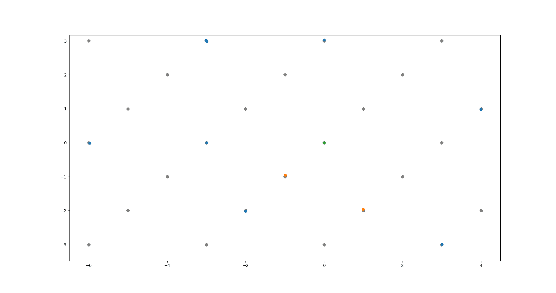
The above image shows the algorithm at work. Green dot is the origin. Grey dots are the underlying lattice (ground truth). Blue dots are the noisy data points the algorithm takes as input. Yellow dots are the lattice basis vectors returned by the algorithm.
code link
https://github.com/pb1729/latticefit
Run lattice_fit.py to get a quick demo.
API: Import lattice_fit and then call lattice_fit(dataset, zeta) where dataset is a 2d numpy array. First index into the dataset selects the datapoint, and the second selects a coordinate of that datapoint. zeta is just a float, whose effect was described above. The result will be an array of basis vectors, sorted from longest to shortest. These will approach zero length at some point, and it's your responsibility as the caller to cut off the list there. (Or perhaps you already know the size of the lattice basis.)
caveats
Admittedly, due to the large (though still polynomial) time complexity of the LLL algorithm, this method scales poorly with the number of data points. The best suggestion I have so far here is just to run the algorithm on manageable subsets of the data, filter out the near-zero vectors, and then run the algorithm again on all the basis vectors found this way.
...
I originally left this as a stack overflow answer that I came across when initially searching for a solution to this problem.
Linkpost for: https://pbement.com/posts/latticefit.html
comment by DaemonicSigil · 2023-10-13T01:27:42.264Z · LW(p) · GW(p)
Very interesting youtube video about the design of multivariate experiments: https://www.youtube.com/watch?v=5oULEuOoRd0 Seems like a very powerful and general tool, yet not too well known.
For people who don't want to click the link, the goal is that we're trying to design experiments where there are many different variables we could change at once. Trying all combinations takes too much effort (too many experiments to run). Changing just one variable at a time completely throws away information about joint effects, plus if there are variables, then only of the data is testing variations of any given variable, which is wasteful, and reduces the sample size.
The key idea (which seems to be called a Taguchi method) is to instead use an orthogonal array to design our experiments. This tries to spread out different settings in a "fairly even" way (see article for precise definition). Then we can figure out the effect of various variables (and even combinations of variables) by grouping our data in different ways after the fact.
comment by DaemonicSigil · 2024-05-05T18:47:46.968Z · LW(p) · GW(p)
Linkpost for: https://pbement.com/posts/threads.html
Today's interesting number is 961.
Say you're writing a CUDA program and you need to accomplish some task for every element of a long array. Well, the classical way to do this is to divide up the job amongst several different threads and let each thread do a part of the array. (We'll ignore blocks for simplicity, maybe each block has its own array to work on or something.) The method here is as follows:
for (int i = threadIdx.x; i < array_len; i += 32) {
    arr[i] = ...;
}
So the threads make the following pattern (if there are threads):
⬛🟫🟥🟧🟨🟩🟦🟪⬛🟫🟥🟧🟨🟩🟦🟪⬛🟫🟥🟧🟨🟩🟦🟪⬛🟫
This is for an array of length . We can see that the work is split as evenly as possible between the threads, except that threads 0 and 1 (black and brown) have to process the last two elements of the array while the rest of the threads have finished their work and remain idle. This is unavoidable because we can't guarantee that the length of the array is a multiple of the number of threads. But this only happens at the tail end of the array, and for a large number of elements, the wasted effort becomes a very small fraction of the total. In any case, each thread will loop times, though it may be idle during the last loop while it waits for the other threads to catch up.
One may be able to spend many happy hours programming the GPU this way before running into a question: What if we want each thread to operate on a continguous area of memory? (In most cases, we don't want this.) In the previous method (which is the canonical one), the parts of the array that each thread worked on were interleaved with each other. Now we run into a scenario where, for some reason, the threads must operate on continguous chunks. "No problem" you say, we simply need to break the array into chunks and give a chunk to each thread.
const int chunksz = (array_len + blockDim.x - 1)/blockDim.x;
for (int i = threadIdx.x*chunksz; i < (threadIdx.x + 1)*chunksz; i++) {
    if (i < array_len) {
        arr[i] = ...;
    }
}
If we size the chunks at 3 items, that won't be enough, so again we need items per chunk. Here is the result:
⬛⬛⬛⬛🟫🟫🟫🟫🟥🟥🟥🟥🟧🟧🟧🟧🟨🟨🟨🟨🟩🟩🟩🟩🟦🟦
Beautiful. Except you may have noticed something missing. There are no purple squares. Though thread 6 is a little lazy and doing 2 items instead of 4, thread 7 is doing absolutely nothing! It's somehow managed to fall off the end of the array.
Unavoidably, some threads must be idle for loops. This is the conserved total amount of idleness. With the first method, the idleness is spread out across threads. Mathematically, the amount of idleness can be no greater than regardless of array length and thread number, and so each thread will be idle for at most 1 loop. But in the contiguous method, the idleness is concentrated in the last threads. There is nothing mathematically impossible about having as big as or bigger, and so it's possible for an entire thread to remain unused. Multiple threads, even. Eg. take :
⬛⬛🟫🟫🟥🟥🟧🟧🟨
3 full threads are unused there! Practically, this shouldn't actually be a problem, though. The number of serial loops is still the same, and the total number of idle loops is still the same. It's just distributed differently. The reasons to prefer the interleaved method to the contiguous method would be related to memory coalescing or bank conflicts. The issue of unused threads would be unimportant.
We don't always run into this effect. If is a multiple of , all threads are fully utilized. Also, we can guarantee that there are no unused threads for larger than a certain maximal value. Namely, take then and so the idleness is . But if is larger than this, then one can show that all threads must be used at least a little bit.
So, if we're using CUDA threads, then when the array size is 961, the contiguous processing method will leave thread 31 idle. And 961 is the largest array size for which that is true.
comment by DaemonicSigil · 2024-02-04T08:50:40.963Z · LW(p) · GW(p)
You Can Just Put an Endpoint Penalty on Your Wasserstein GAN
Linkpost for: https://pbement.com/posts/endpoint_penalty.html
When training a Wasserstein GAN, there is a very important constraint that the discriminator network must be a Lipschitz-continuous function. Roughly we can think of this as saying that the output of the function can't change too fast with respect to position, and this change must be bounded by some constant . If the discriminator function is given by then we can write the Lipschitz condition for the discriminator as:
Usually this is implemented as a gradient penalty. People will take a gradient (higher order, since the loss already has a gradient in it) of this loss (for ):
In this expression is sampled as , a random mixture of a real and a generated data point.
But this is complicated to implement, involving a higher order gradient. It turns out we can also just impose the Lipschitz condition directly, via the following penalty:
Except to prevent issues where we're maybe sometimes dividing by zero, we throw in an and a reweighting factor of (not sure if that is fully necessary, but the intuition is that making sure the Lipschitz condition is enforced for points at large separation is the most important thing).
For the overall loss, we compare all pairwise distances between real data and generated data and a random mixture of them. Probably it improves things to add 1 or two more random mixtures in, but I'm not sure and haven't tried it.
In any case, this seems to work decently well (tried on mnist), so it might be a simpler alternative to gradient penalty. I also used instance noise, which as pointed out here, is amazingly good for preventing mode collapse and just generally makes training easier. So yeah, instance noise is great and you should use it. And if you really don't want to figure out how to do higher order gradients in pytorch for your WGAN, you've still got options.