Beyond Gaussian: Language Model Representations and Distributions
post by Matt Levinson · 2024-11-24T01:53:38.156Z · LW · GW · 1 commentsContents
  Logistic Dominated Mixture Distribution
  Representational Vector Similarities
  Future Work
None
1 comment
In January 2023, beren and Eric Winsor cataloged basic distributional properties [LW · GW] of weights, activations, and gradients in GPT-2 models, providing a systematic view of model internals (thanks to Ryan Greenblatt for the pointer). This post extends their investigation in two directions.
First, examining their characterization of transformer activations as "nearly Gaussian with outliers," I conducted detailed distributional analyses of post-residual activations. Myfindings align with observations made in comments and unpublished work: the distributions are better described by heavier-tailed distributions, dominated by the logistic distribution. What can appears as outliers or artifacts manifests in my analysis as consistent mixture distributions, with minor modes appearing systematically to both sides of the primary distribution.
Second, prompted by Buck at Redwood Research (who shared initial code), I investigated how different aspects of language - subjects, attributes, and styles - interact in the model's representational space. I analyzed the relative distances between representations of sentences varying in subject matter and attributes (like tone or language) and found some patterns in how these characteristics compete for dominance in the model's internal representations. Perhaps most interesting, there is a consistent diminishing of these distances through the model's layers. Overall I had ten subjects, twelve attributes, and 200 sentences for each pair generated by Claude 3.5 Sonnet (before the update a few weeks ago). This is the dataset used for all of the work presented here.
Below I’ll run through some of the most intriguing patterns I found and some thoughts on potential future directions. I do not expect distributional analysis to become a primary tool in safety or interpretability. My goal is to contribute to the higher level characterization of transformer based LLMs. My hope is that such characterization may suggest directions for future work that can contribute directly to safety and interpretability goals. I’d be interested to hear from the community if you have any questions or thoughts about future work.
Logistic Dominated Mixture Distribution
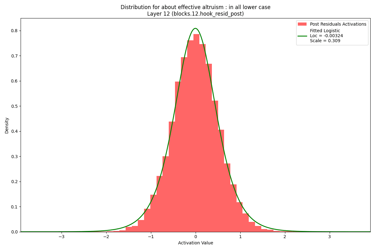
The logistic distribution dominated. I fit a range of distributions to the concatenation of the post-residual activations at each layer for each subject:attribute pair for GPT2-Small, GPT2-Medium, GPT2-Large, Pythia-160m, Pythia-410m, and Pythia-1b. For the Pythia models, the logistic and related distributions (generalized logistic and hyperbolic secant) dominated with the best fit 85% of the time, increasing slightly from 160m to 1b. The remainder were split evenly between lighter and heavier tails, with the generalized normal or crystal ball distributions fitting best 4.7% of the time and the t-distribution with degrees of freedom between 2 and 3.7 fitting best 7.4% of the time. For the GPT2 models, the heavy tails of the t-distribution with low degrees of freedom was much more common, representing 37% of distributions. The other 63% were best fit by the mid-weight tailed distribution, logistic, generalized logistic, and hyperbolic secant, 67% of the time. The only outlier is the final layer of the Pythia-160m model, where the post-residual activations were almost perfectly symmetrically bimodal!
This suggests the common approach of using Gaussian mixture modeling for anomaly detection might not be the best. While theoretically GMMs can fit any distribution with enough elements in the mixture, one could certainly be more efficient, and likely more accurate, using mixture components that match the known shape of the target distribution better. Below is a typical example from the Pythia-410m model. Note there are no point mass outliers as reported in the previous work noted above. I did not see these in the GPT2 models examined in that work either.
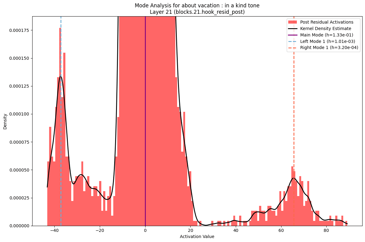
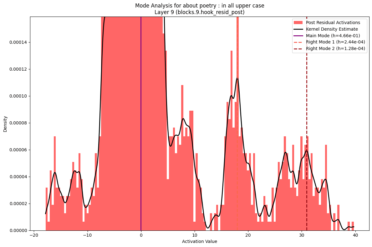
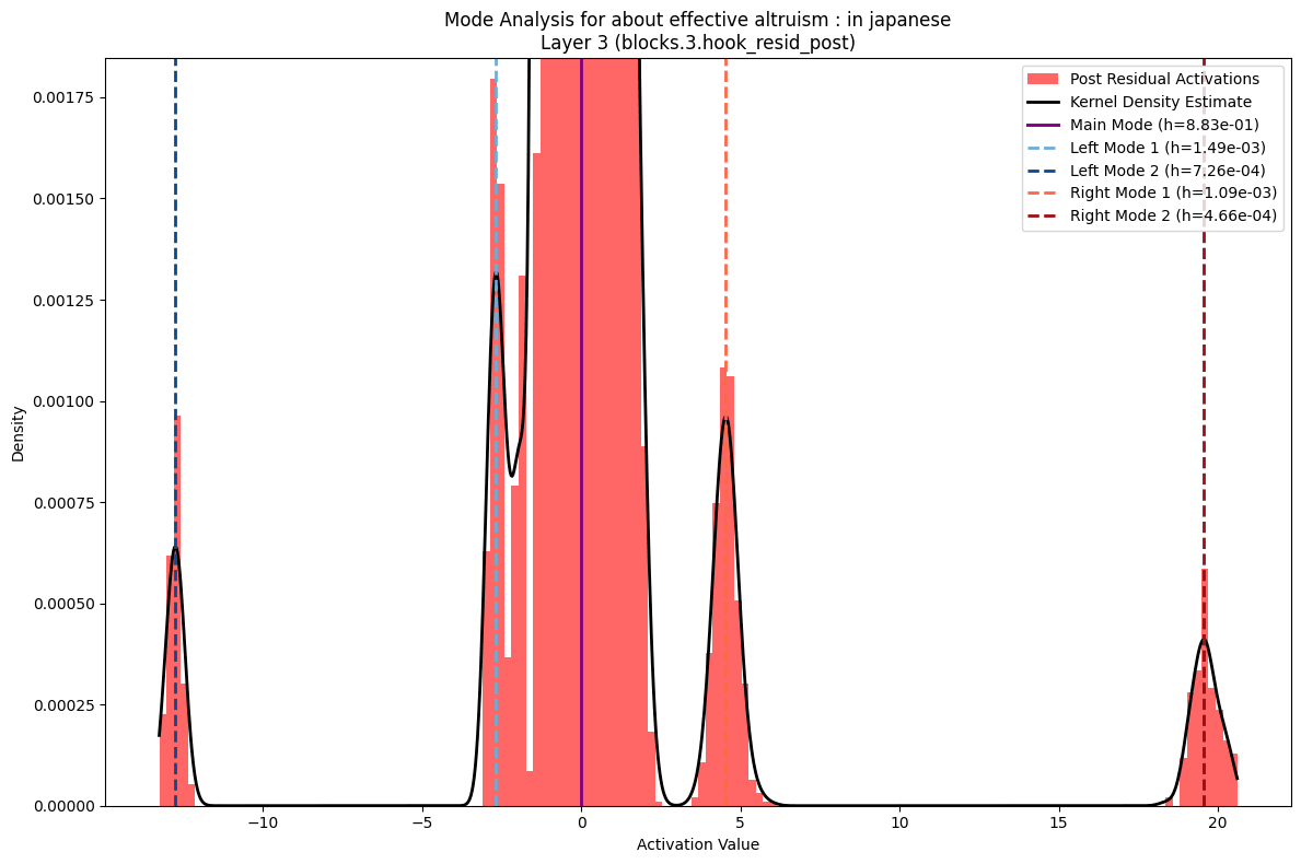
More interesting is what you see if you zoom in. To both sides of the primary distribution you see what are small but clear secondary modes. To analyze these I fit a kernel density estimate to the data and then used the peak finder in scipy.signal. I played with the parameters to bias towards false negatives versus false positives. You can see a few probably missed secondary modes in the examples below.
Some models had more secondary nodes on the left while others had more secondary modes on the right. There was a general pattern of a fairly constant number of nodes on the right, while the number of left modes tended to decrease as you got deeper into the model.
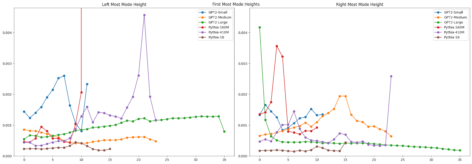
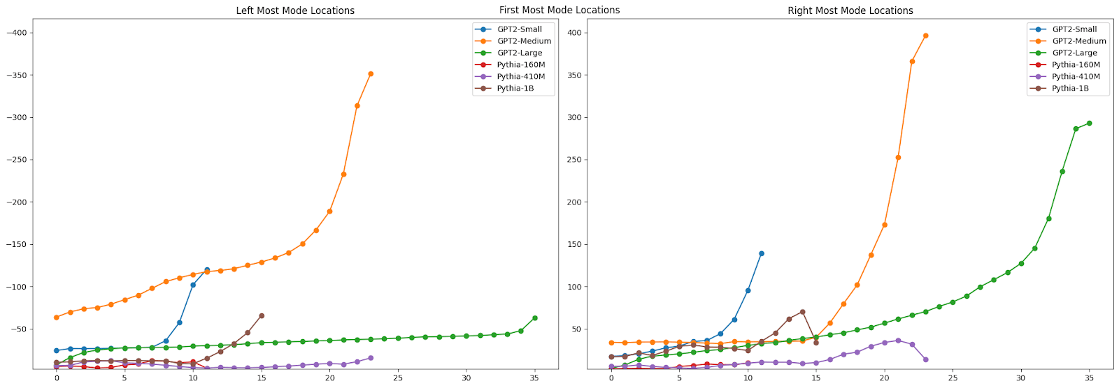
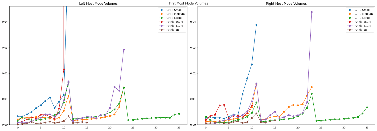
Some other interesting patterns emerged. There are clear shifts in mode height, location, and volume (calculated as the estimated peak height time peak spread) across layers. We see interesting points where the pattern is consistent across models, where in other places there is no consistent pattern across models.
If you look more closely at the distribution of mode characteristics across layers, you see some interesting patterns there as well. The GPT2-Medium model, for example, shows a bimodal distribution of the distance from the center of the left-most mode, with one mode dominating early layers and another taking over in later layers. This transition, along with corresponding shifts in mode heights, might mark key points where the model's representation strategy changes - perhaps reflecting different stages of linguistic processing.
There were also some interesting patterns when looking at sentence attributes. Picking out the pattern across layers and attributes is a potential place for further work. But there are clearly some interesting things going on. Most strikingly, sentences in Japanese had clearer, more distinct secondary modes across models. This tended to be clearer in earlier layers, but mostly held throughout in the visual examinations I've done. The persistence of these distinct modes might reflect how the model maintains separate computational channels for handling the fundamentally different linguistic structures of Japanese, even as it integrates semantic information across languages. This example is typical of earlier layers.
Representational Vector Similarities
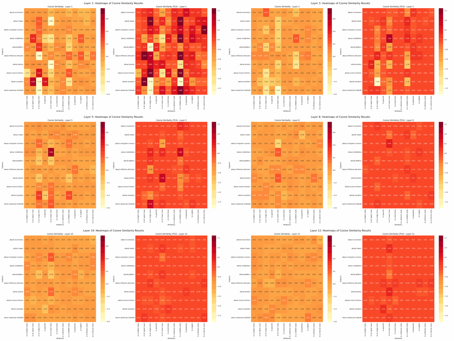
This work kicked off with the question noted above posed by Buck at Redwood Research. This work was limited to the GPT2-Small model. I designed my analysis to find whether a particular subject or attribute was represented in a unique direction more strongly than other subjects or attributes. To do this, I took a subject, call it s1, and an attribute, a1. Then across all pairs of subjects including s1 and all pairs of attributes including a1, I measured the cosine similarity of the post residual vector at each layer for sentences with the subject:attribute pair s1a2 versus those for s1a1 sentences and s2a2 sentences. I did likewise for s2a1 sentences. Across all sets of sentences and attributes, I took the average difference in cosine similarity for the comparisons. In this way we can see whether a subject or attribute is more distinctive or attracting. In the gif below, positive numbers mean the subject was more attracting, while negative numbers mean the opposite. I did this analysis with both the raw residuals and ones reduced in dimension via PCA to represent 90% of the variance of the vectors. When the dimension is so high and can be reduced by an order of magnitude while conserving the large majority of variance, I tend to believe the PCA versions more. But I have not done deep validation. In either case, you’ll see that the attributes in an angry tone, in all lower case, and in a childish style most consistently attract or repulse. You can also see a systematic decrease in subject/attribute distinctiveness as we traverse through the model. Perhaps this decrease across layers hints at how the model progressively abstracts and combines features? The fact that certain attributes like in all lower case maintain stronger distinctiveness even in later layers might suggest which features remain fundamental even as the model moves towards final encoding and prediction?
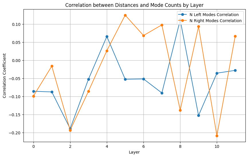
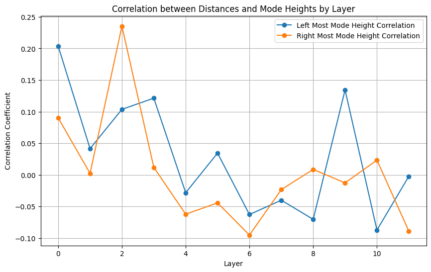
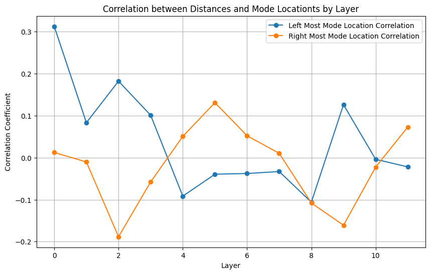
Finally, I took a first pass at examining the interconnection between this specific analysis of internal representations and the distributional analysis described above. I simply looked at correlations between some of the mode characteristics and the differentials in the heatmap.
You can see some patterns here that could warrant further investigation. Expanding this analysis from GPT2-Small to the rest of the models in the distributional analysis could reveal broader patterns. Are there hints here that distributional information could augment other tools in interpretability discovery?
Future Work
As to potential future direction, I’m interested in thoughts from the community as I’m newer to the AI safety and interpretability space. I see potential future work in a few areas.
One promising direction is anomaly detection. As noted above, the heavier-tailed nature of most of these distributions suggests current Gaussian-based approaches might be missing important structure. For instance, a model that leverages heavier tailed distributions and explicitly accounts for minor modes might better distinguish between normal variation and genuinely anomalous activations..
The presence of consistent minor modes also raises intriguing possibilities for interpretability work. Rather than analyzing predetermined categories like the subject-attribute pairs used here, we could potentially use mode characteristics to discover meaningful subspaces in an unsupervised way. For example, the fact that Japanese text produces distinctly stronger secondary modes suggests these features might help identify specialized computational channels. Could this complement existing circuit discovery techniques by providing additional signals for where to look for specialized functionality? It could also be illuminating to see how this analysis might change when considering residual vectors which have been projected into higher dimension through sparse autoencoders.
1 comments
Comments sorted by top scores.
comment by Matt Levinson · 2024-12-02T21:13:27.157Z · LW(p) · GW(p)
I've uploaded the code to github.
