Improving Dictionary Learning with Gated Sparse Autoencoders
post by Senthooran Rajamanoharan (SenR), Arthur Conmy (arthur-conmy), lewis smith (lsgos), Tom Lieberum (Frederik), Vikrant Varma (amrav), János Kramár (janos-kramar), Rohin Shah (rohinmshah), Neel Nanda (neel-nanda-1) · 2024-04-25T18:43:47.003Z · LW · GW · 38 commentsThis is a link post for https://arxiv.org/abs/2404.16014
Contents
38 comments
Authors: Senthooran Rajamanoharan*, Arthur Conmy*, Lewis Smith, Tom Lieberum, Vikrant Varma, János Kramár, Rohin Shah, Neel Nanda
A new paper from the Google DeepMind mech interp team: Improving Dictionary Learning with Gated Sparse Autoencoders!
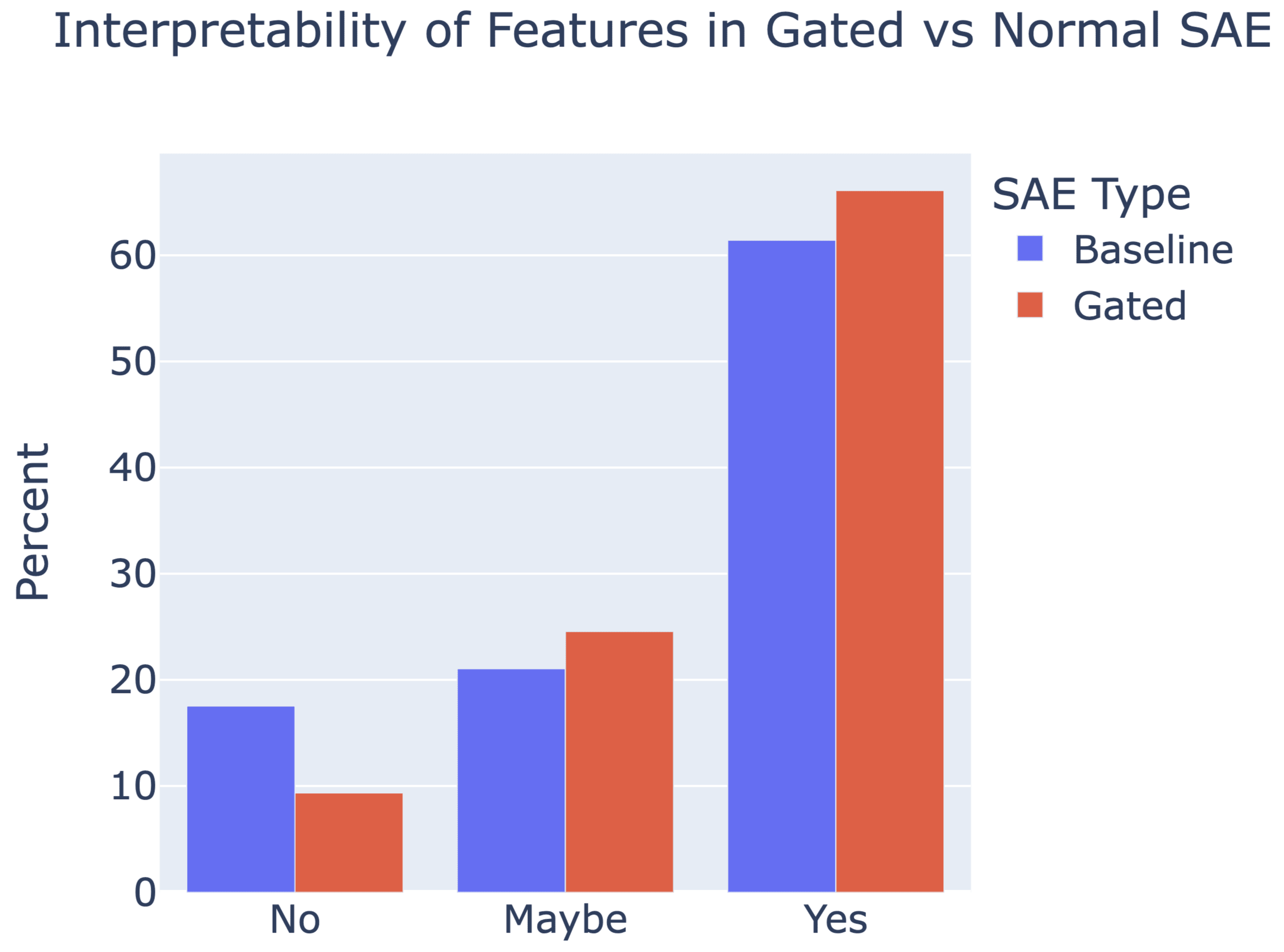
Gated SAEs are a new Sparse Autoencoder architecture that seems to be a significant Pareto-improvement over normal SAEs, verified on models up to Gemma 7B. They are now our team's preferred way to train sparse autoencoders, and we'd love to see them adopted by the community! (Or to be convinced that it would be a bad idea for them to be adopted by the community!)

They achieve similar reconstruction with about half as many firing features, and while being either comparably or more interpretable (confidence interval for the increase is 0%-13%).
See Sen's Twitter summary, my Twitter summary, and the paper!
38 comments
Comments sorted by top scores.
comment by Sam Marks (samuel-marks) · 2024-04-25T20:55:25.702Z · LW(p) · GW(p)
Great work! Obviously the results here speak for themselves, but I especially wanted to complement the authors on the writing. I thought this paper was a pleasure to read, and easily a top 5% exemplar of clear technical writing. Thanks for putting in the effort on that.
I'll post a few questions as children to this comment.
Replies from: samuel-marks, samuel-marks, samuel-marks, neel-nanda-1↑ comment by Sam Marks (samuel-marks) · 2024-04-25T21:12:52.537Z · LW(p) · GW(p)
I believe that equation (10) giving the analytical solution to the optimization problem defining the relative reconstruction bias is incorrect. I believe the correct expression should be .
You could compute this by differentiating equation (9), setting it equal to 0 and solving for . But here's a more geometrical argument.
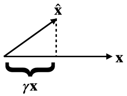
By definition, is the multiple of closest to . Equivalently, this closest such vector can be described as the projection . Setting these equal, we get the claimed expression for .
As a sanity check, when our vectors are 1-dimensional, , and , we my expression gives (which is correct), but equation (10) in the paper gives .
Replies from: arthur-conmy↑ comment by Arthur Conmy (arthur-conmy) · 2024-04-25T21:29:38.307Z · LW(p) · GW(p)
Oh oops, thanks so much. We'll update the paper accordingly. Nit: it's actually
(it's just minimizing a quadratic)
ETA: the reason we have complicated equations is that we didn't compute during training (this quantity is kinda weird). However, you can compute from quantities that are usually tracked in SAE training. Specifically, and all terms here are clearly helpful to track in SAE training.
↑ comment by Sam Marks (samuel-marks) · 2024-04-25T22:13:00.663Z · LW(p) · GW(p)
Oh, one other issue relating to this: in the paper it's claimed that if is the argmin of then is the argmin of . However, this is not actually true: the argmin of the latter expression is . To get an intuition here, consider the case where and are very nearly perpendicular, with the angle between them just slightly less than . Then you should be able to convince yourself that the best factor to scale either or by in order to minimize the distance to the other will be just slightly greater than 0. Thus the optimal scaling factors cannot be reciprocals of each other.
ETA: Thinking on this a bit more, this might actually reflect a general issue with the way we think about feature shrinkage; namely, that whenever there is a nonzero angle between two vectors of the same length, the best way to make either vector close to the other will be by shrinking it. I'll need to think about whether this makes me less convinced that the usual measures of feature shrinkage are capturing a real thing.
ETA2: In fact, now I'm a bit confused why your figure 6 shows no shrinkage. Based on what I wrote above in this comment, we should generally expect to see shrinkage (according to the definition given in equation (9)) whenever the autoencoder isn't perfect. I guess the answer must somehow be "equation (10) actually is a good measure of shrinkage, in fact a better measure of shrinkage than the 'corrected' version of equation (10)." That's pretty cool and surprising, because I don't really have a great intuition for what equation (10) is actually capturing.
Replies from: rohinmshah, SenR↑ comment by Rohin Shah (rohinmshah) · 2024-04-25T22:54:11.997Z · LW(p) · GW(p)
Thinking on this a bit more, this might actually reflect a general issue with the way we think about feature shrinkage; namely, that whenever there is a nonzero angle between two vectors of the same length, the best way to make either vector close to the other will be by shrinking it.
This was actually the key motivation for building this metric in the first place, instead of just looking at the ratio . Looking at the that would optimize the reconstruction loss ensures that we're capturing only bias from the L1 regularization, and not capturing the "inherent" need to shrink the vector given these nonzero angles. (In particular, if we computed for Gated SAEs, I expect that would be below 1.)
I think the main thing we got wrong is that we accidentally treated as though it were . To the extent that was the main mistake, I think it explains why our results still look how we expected them to -- usually is going to be close to 1 (and should be almost exactly 1 if shrinkage is solved), so in practice the error introduced from this mistake is going to be extremely small.
We're going to take a closer look at this tomorrow, check everything more carefully, and post an update after doing that. I think it's probably worth waiting for that -- I expect we'll provide much more detailed derivations that make everything a lot clearer.
↑ comment by Senthooran Rajamanoharan (SenR) · 2024-04-25T22:57:22.598Z · LW(p) · GW(p)
Hey Sam, thanks - you're right. The definition of reconstruction bias is actually the argmin of
which I'd (incorrectly) rearranged as the expression in the paper. As a result, the optimum is
That being said, the derivation we gave was not quite right, as I'd incorrectly substituted the optimised loss rather than the original reconstruction loss, which makes equation (10) incorrect. However the difference between the two is small exactly when gamma is close to one (and indeed vanishes when there is no shrinkage), which is probably why we didn't pick this up. Anyway, we plan to correct these two equations and update the graphs, and will submit a revised version.
Replies from: SenR↑ comment by Senthooran Rajamanoharan (SenR) · 2024-04-26T12:38:44.850Z · LW(p) · GW(p)
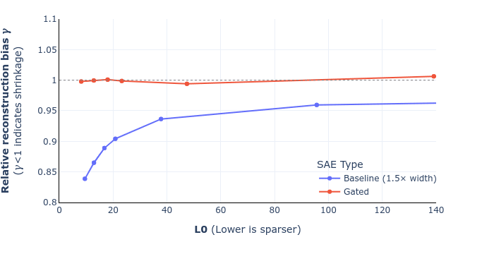
UPDATE: we've corrected equations 9 and 10 in the paper (screenshot of the draft below) and also added a footnote that hopefully helps clarify the derivation. I've also attached a revised figure 6, showing that this doesn't change the overall story (for the mathematical reasons I mentioned in my previous comment). These will go up on arXiv, along with some other minor changes (like remembering to mention SAEs' widths), likely some point next week. Thanks again Sam for pointing this out!
Updated equations (draft):

Updated figure 6 (shrinkage comparison for GELU-1L):
↑ comment by Sam Marks (samuel-marks) · 2024-04-25T21:36:02.353Z · LW(p) · GW(p)
I'm a bit perplexed by the choice of loss function for training GSAEs (given by equation (8) in the paper). The intuitive (to me) thing to do here would be would be to have the and terms, but not the term, since the point of is to tell you which features should be active, not to itself provide good feature coefficients for reconstructing . I can sort of see how not including this term might result in the coordinates of all being extremely small (but barely positive when it's appropriate to use a feature), such that the sparsity term doesn't contribute much to the loss. Is that what goes wrong? Are there ablation experiments you can report for this? If so, including this term still currently seems to me like a pretty unprincipled way to deal with this -- can the authors provide any flavor here?
Here are two ways that I've come up with for thinking about this loss function -- let me know if either of these are on the right track. Let denote the gated encoder, but with a ReLU activation instead of Heaviside. Note then that is just the standard SAE encoder from Towards Monosemanticity.
Perspective 1: The usual loss from Towards Monosemanticity for training SAEs is (this is the same as your and up to the detaching thing). But now you have this magnitude network which needs to get a gradient signal. Let's do that by adding an additional term -- your . So under this perspective, it's the reconstruction term which is new, with the sparsity and auxiliary terms being carried over from the usual way of doing things.
Perspective 2 (h/t Jannik Brinkmann): let's just add together the usual Towards Monosemanticity loss function for both the usual architecture and the new modified archiecture: .
However, the gradients with respect to the second term in this sum vanish because of the use of the Heaviside, so the gradient with respect to this loss is the same as the gradient with respect to the loss you actually used.
Replies from: rohinmshah↑ comment by Rohin Shah (rohinmshah) · 2024-04-25T21:52:45.883Z · LW(p) · GW(p)
Possibly I'm missing something, but if you don't have , then the only gradients to and come from (the binarizing Heaviside activation function kills gradients from ), and so would be always non-positive to get perfect zero sparsity loss. (That is, if you only optimize for L1 sparsity, the obvious solution is "none of the features are active".)
(You could use a smooth activation function as the gate, e.g. an element-wise sigmoid, and then you could just stick with from the beginning of Section 3.2.2.)
↑ comment by Sam Marks (samuel-marks) · 2024-04-25T21:57:17.533Z · LW(p) · GW(p)
Ah thanks, you're totally right -- that mostly resolves my confusion. I'm still a little bit dissatisfied, though, because the term is optimizing for something that we don't especially want (i.e. for to do a good job of reconstructing ). But I do see how you do need to have some sort of a reconstruction-esque term that actually allows gradients to pass through to the gated network.
Replies from: SenR↑ comment by Senthooran Rajamanoharan (SenR) · 2024-04-25T23:08:32.041Z · LW(p) · GW(p)
Yep, the intuition here indeed was that L1 penalised reconstruction seems to be okay for teaching a standard SAE's encoder to detect which features are on (even if features get shrunk as a result), so that is effectively what this auxiliary loss is teaching the gate sub-layer to do, alongside the sparsity penalty. (The key difference being we freeze the decoder in the auxiliary task, which the ablation study shows helps performance.) Maybe to put it another way, this was an auxiliary task that we had good evidence would teach the gate sublayer to detect active features reasonably well, and it turned out to give good results in practice. It's totally possible though that there are better auxiliary tasks (or even completely different loss functions) out there that we've not explored.
↑ comment by Sam Marks (samuel-marks) · 2024-04-25T21:52:20.572Z · LW(p) · GW(p)
(The question in this comment is more narrow and probably not interesting to most people.)
The limitations section includes this paragraph:
One worry about increasing the expressivity of sparse autoencoders is that they will overfit when
reconstructing activations (Olah et al., 2023, Dictionary Learning Worries), since the underlying
model only uses simple MLPs and attention heads, and in particular lacks discontinuities such as step
functions. Overall we do not see evidence for this. Our evaluations use held-out test data and we
check for interpretability manually. But these evaluations are not totally comprehensive: for example,
they do not test that the dictionaries learned contain causally meaningful intermediate variables in the
model’s computation. The discontinuity in particular introduces issues with methods like integrated
gradients (Sundararajan et al., 2017) that discretely approximate a path integral, as applied to SAEs
by Marks et al. (2024).
I'm not sure I understand the point about integrated gradients here. I understand this sentence as meaning: since model outputs are a discontinuous function of feature activations, integrated gradients will do a bad job of estimating the effect of patching feature activations to counterfactual values.
If that interpretation is correct, then I guess I'm confused because I think IG actually handles this sort of thing pretty gracefully. As long as the number of intermediate points you're using is large enough that you're sampling points pretty close to the discontinuity on both sides, then your error won't be too large. This is in contrast to attribution patching which will have a pretty rough time here (but not really that much worse than with the normal ReLU encoders, I guess). (And maybe you also meant for this point to apply to attribution patching?)
Replies from: neel-nanda-1↑ comment by Neel Nanda (neel-nanda-1) · 2024-04-26T00:14:38.219Z · LW(p) · GW(p)
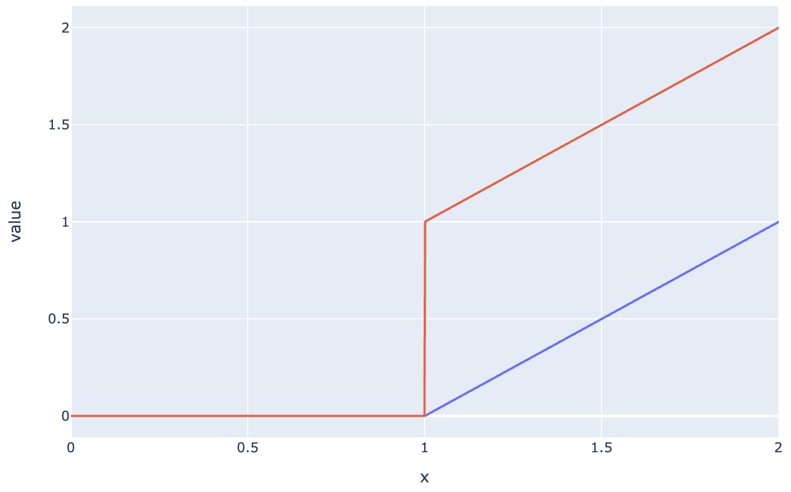
I haven't fully worked through the maths, but I think both IG and attribution patching break down here? The fundamental problem is that the discontinuity is invisible to IG because it only takes derivatives. Eg the ReLU and Jump ReLU below look identical from the perspective of IG, but not from the perspective of activation patching, I think.
↑ comment by Sam Marks (samuel-marks) · 2024-04-26T00:36:58.112Z · LW(p) · GW(p)
Yep, you're totally right -- thanks!
↑ comment by Neel Nanda (neel-nanda-1) · 2024-04-25T21:03:42.881Z · LW(p) · GW(p)
Great work! Obviously the results here speak for themselves, but I especially wanted to complement the authors on the writing. I thought this paper was a pleasure to read, and easily a top 5% exemplar of clear technical writing. Thanks for putting in the effort on that.
<3 Thanks so much, that's extremely kind. Credit entirely goes to Sen and Arthur, which is even more impressive given that they somehow took this from a blog post to a paper in a two week sprint! (including re-running all the experiments!!)
comment by Dan Braun (dan-braun-1) · 2024-04-26T08:44:32.809Z · LW(p) · GW(p)
This is neat, nice work!
I'm finding it quite hard to get a sense at what the actual Loss Recovered numbers you report are, and to compare them concretely to other work. If possible, it'd be very helpful if you shared:
- What the zero ablations CE scores are for each model and SAE position. (I assume it's much worse for the MLP and attention outputs than the residual stream?)
- What the baseline CE scores are for each model.
↑ comment by Arthur Conmy (arthur-conmy) · 2024-04-29T18:17:07.159Z · LW(p) · GW(p)
Thanks for the feedback, we will put up an update to the paper with all these numbers in tables, tomorrow night. For now I have sent you them (and can send anyone else them who wants them in the next 24H)
comment by leogao · 2024-04-26T01:28:42.734Z · LW(p) · GW(p)
Great paper! The gating approach is an interesting way to learn the JumpReLU threshold and it's exciting that it works well. We've been working on some related directions at OpenAI based on similar intuitions about feature shrinking.
Some questions:
- Is b_mag still necessary in the gated autoencoder?
- Did you sweep learning rates for the baseline and your approach?
- How large is the dictionary of the autoencoder?
↑ comment by Arthur Conmy (arthur-conmy) · 2024-04-27T00:03:26.936Z · LW(p) · GW(p)
We use learning rate 0.0003 for all Gated SAE experiments, and also the GELU-1L baseline experiment. We swept for optimal baseline learning rates on GELU-1L for the baseline SAE to generate this value.
For the Pythia-2.8B and Gemma-7B baseline SAE experiments, we divided the L2 loss by , motivated by wanting better hyperparameter transfer, and so changed learning rate to 0.001 or 0.00075 for all the runs (currently in Figure 1, only attention output pre-linear uses 0.00075. In the rerelease we'll state all the values used). We didn't see noticable difference in the Pareto frontier changing between 0.001 and 0.00075 so did not sweep the baseline hyperparameter further than this.
Replies from: leogao↑ comment by Neel Nanda (neel-nanda-1) · 2024-04-26T02:48:49.168Z · LW(p) · GW(p)
Re dictionary width, 2**17 (~131K) for most Gated SAEs, 3*(2**16) for baseline SAEs, except for the (Pythia-2.8B, Residual Stream) sites we used 2**15 for Gated and 3*(2**14) for baseline since early runs of these had lots of feature death. (This'll be added to the paper soon, sorry!). I'll leave the other Qs for my co-authors
Replies from: leogao↑ comment by leogao · 2024-05-01T00:01:29.377Z · LW(p) · GW(p)
Got it - do you think with a bit more tuning the feature death at larger scale could be eliminated, or would it be tough to manage with the reinitialization approach?
Replies from: arthur-conmy↑ comment by Arthur Conmy (arthur-conmy) · 2024-05-01T00:49:14.596Z · LW(p) · GW(p)
I'm not sure what you mean by "the reinitialization approach" but feature death doesn't seem to be a major issue at the moment. At all sites besides L27, our Gemma-7B SAEs didn't have much feature death at all (stats at https://arxiv.org/pdf/2404.16014v2 up in a few hours), and also the Anthropic update suggests even in small models the problem can be addressed.
Replies from: leogao↑ comment by leogao · 2024-05-01T01:01:34.818Z · LW(p) · GW(p)
Sorry I meant the Anthropiclike neuron resampling procedure.
I think I misread Neel's comment, I thought he was saying that 131k was chosen because larger autoencoders would have too many dead latents (as opposed to this only being for Pythia residual).
Replies from: arthur-conmy↑ comment by Arthur Conmy (arthur-conmy) · 2024-05-01T01:06:04.838Z · LW(p) · GW(p)
Ah yeah, Neel's comment makes no claims about feature death beyond Pythia 2.8B residual streams. I trained 524K width Pythia-2.8B MLP SAEs with <5% feature death (not in paper), and Anthropic's work gets to >1M live features (with no claims about interpretability) which together would make me surprised if 131K was near the max of possible numbers of live features even in small models.
↑ comment by Senthooran Rajamanoharan (SenR) · 2024-04-29T08:51:51.922Z · LW(p) · GW(p)
On , it's unclear what a "natural" choice would be for setting this parameter in order to simplify the architecture further. One natural reference point is to set it to , but this corresponds to getting rid of the discontinuity in the Jump ReLU (turning the magnitude encoder into a ReLU on multiplicatively rescaled gate encoder preactivations). Effectively (removing the now unnecessary auxiliary task), this would give results similar to the "baseline + rescale & shift" benchmark in section 5.2 of the paper, although probably worse, as we wouldn't have the shift.
Replies from: leogaocomment by Charlie Steiner · 2024-04-25T22:19:01.069Z · LW(p) · GW(p)
Nice. I tried to do something similar (except making everything leaky with polynomial tails, so
y = (y+torch.sqrt(y**2+scale**2)) * (1+(y+threshold)/torch.sqrt((y+threshold)**2+scale**2)) / 4
where the first part (y+torch.sqrt(y**2+scale**2)) is a softplus, and the second part (1+(y+threshold)/torch.sqrt((y+threshold)**2+scale**2)) is a leaky cutoff at the value threshold.
But I don't think I got such clearly better results, so I'm going to have to read more thoroughly to see what else you were doing that I wasn't :)
comment by leogao · 2024-05-01T00:04:50.628Z · LW(p) · GW(p)
Another question: any particular reason to expect ablate-to-zero to be the most relevant baseline? In my experiments, I find ablate to zero to completely destroy the loss. So it's unclear whether 90% recovered on this metric actually means that much - GPT-2 probably recovers 90% of the loss of GPT-4 under this metric, but obviously GPT-2 only explains a tiny fraction of GPT-4's capabilities. I feel like a more natural measure may be for example the equivalent compute efficiency hit.
Replies from: neel-nanda-1, arthur-conmy↑ comment by Neel Nanda (neel-nanda-1) · 2024-05-01T01:03:47.189Z · LW(p) · GW(p)
Nah I think it's pretty sketchy. I personally prefer mean ablation, especially for residual stream SAEs where zero ablation is super damaging. But even there I agree. Compute efficiency hit would be nice, though it's a pain to get the scaling laws precise enough
For our paper this is irrelevant though IMO because we're comparing gated and normal SAEs, and I think this is just scaling by a constant? It's at least monotonic in CE loss degradation
↑ comment by Arthur Conmy (arthur-conmy) · 2024-05-01T01:02:38.982Z · LW(p) · GW(p)
I don't think zero ablation is that great a baseline. We're mostly using it for continuity's sake with Anthropic's prior work (and also it's a bit easier to explain than a mean ablation baseline which requires specifying where the mean is calculated from). In the updated paper https://arxiv.org/pdf/2404.16014v2 (up in a few hours) we show all the CE loss numbers for anyone to scale how they wish.
I don't think compute efficiency hit[1] is ideal. It's really expensive to compute, since you can't just calculate it from an SAE alone as you need to know facts about smaller LLMs. It also doesn't transfer as well between sites (splicing in an attention layer SAE doesn't impact loss much, splicing in an MLP SAE impacts loss more, and residual stream SAEs impact loss the most). Overall I expect it's a useful expensive alternative to loss recovered, not a replacement.
EDIT: on consideration of Leo's reply, I think my point about transfer is wrong; a metric like "compute efficiency recovered" could always be created by rescaling the compute efficiency number.
- ^
What I understand "compute efficiency hit" to mean is: for a given (SAE, ) pair, how much less compute you'd need (as a multiplier) to train a different LM, such that gets the same loss as -with-the-SAE-spliced-in.
↑ comment by leogao · 2024-05-01T01:08:21.989Z · LW(p) · GW(p)
It doesn't seem like a huge deal to depend on the existence of smaller LLMs - they'll be cheap compared to the bigger one, and many LM series already contain smaller models. Not transferring between sites seems like a problem for any kind of reconstruction based metric because there's actually just differently important information in different parts of the model.
comment by J Bostock (Jemist) · 2024-05-30T15:14:18.160Z · LW(p) · GW(p)
Is there a solution to avoid constraining the norms of the columns of to be 1? Anthropic report better results when letting it be unconstrained. I've tried not constraining it and allowing it to vary which actually gives a slight speedup in performance. This also allows me to avoid an awkward backward hook. Perhaps most of the shrinking effect gets absorbed by the term?
Replies from: SenR↑ comment by Senthooran Rajamanoharan (SenR) · 2024-05-31T08:47:34.164Z · LW(p) · GW(p)
Good question - we're planning to post an update on this point about combining the new sparsity penalty from Anthropic with Gated SAEs. The TL;DR is that you can replace the L1 term in the Gated SAE loss with the analogous (gated feature magnitudes dotted with decoder magnitudes) sparsity term introduced by Anthropic and thereby do away with the decoder norms constraint and resampling. If you're going to do this, you also need to either unfreeze the decoder in the auxiliary task, or freeze the decoder weights where they appear in the sparsity penalty; both attain reasonably similar performance, and are definitely better than having the decoder weights frozen in one place but not the other. Put together, this seems to a marginal hit (versus the original Gated loss with L1 penalty and resampling) when comparing Pareto curves, but may be worth to the extent it simplifies training (with this loss function, the SAE training loop just becomes a vanilla neural network training loop).
PS With either the original (L1-based) loss or the modified loss of the previous paragraph, some of the other improvements suggested in the Anthropic post -- in particular, initializing the encoder weights to the transpose of the decoder weights (only at initialisation, not tying them thereafter), and warming up lambda. My point about the new loss not being Pareto better than L1 applies only if you compare like with like -- i.e. apply these other improvements in both cases.
comment by fvncc · 2024-04-26T00:47:49.550Z · LW(p) · GW(p)
Hi any idea how this would compare to just replacing the loss with a smoothed loss function? Something like (summed across the sparse representation).
Replies from: SenR↑ comment by Senthooran Rajamanoharan (SenR) · 2024-05-31T08:57:46.380Z · LW(p) · GW(p)
We found that exactly that form of sparsity penalty did improve shrinkage with standard (ungated) SAEs, and provide a decent boost to loss recovered at low L0. (We didn't evaluate interpretability though.) But then we hit upon Gated SAEs which looked even better, and for which modifying the sparsity penalty in this way feels less necessary, so we haven't experimented with combining the two.
comment by jacob_drori (jacobcd52) · 2024-04-26T00:00:08.730Z · LW(p) · GW(p)
Nice work! I'm not sure I fully understand what the "gated-ness" is adding, i.e. what the role the Heaviside step function is playing. What would happen if we did away with it? Namely, consider this setup:
Let and be the encoder and decoder functions, as in your paper, and let be the model activation that is fed into the SAE.
The usual SAE reconstruction is , which suffers from the shrinkage problem.
Now, introduce a new learned parameter , and define an "expanded" reconstruction , where denotes elementwise multiplication.
Finally, take the loss to be:
.
where ensures the decoder gets no gradients from the first term. As I understand it, this is exactly the loss appearing in your paper. The only difference in the setup is the lack of the Heaviside step function.
Did you try this setup? Or does it fail for an obvious reason I missed?
Replies from: rohinmshah↑ comment by Rohin Shah (rohinmshah) · 2024-04-26T06:50:24.121Z · LW(p) · GW(p)
This suggestion seems less expressive than (but similar in spirit to) the "rescale & shift" baseline we compare to in Figure 9. The rescale & shift baseline is sufficient to resolve shrinkage, but it doesn't capture all the benefits of Gated SAEs.
The core point is that L1 regularization adds lots of biases, of which shrinkage is just one example, so you want to localize the effect of L1 as much as possible. In our setup L1 applies to , so you might think of as "tainted", and want to use it as little as possible. The only thing you really need L1 for is to deter the model from setting too many features active, i.e. you need it to apply to one bit per feature (whether that feature is on / off). The Heaviside step function makes sure we are extracting just that one bit, and relying on for everything else.