[Aspiration-based designs] A. Damages from misaligned optimization – two more models

post by Jobst Heitzig, Simon Dima (simon-dima) · 2024-07-15T14:08:15.716Z · LW · GW · 0 comments

Contents

  Model 1: Purchasing goods
    Introduction: Two-good tradeoffs
    Full model
    Big losses from forgotten values
    Average utility loss
    Numerical evidence for Goodhart effect
  Model 2: Utility estimation from rankings of samples
    State space, true utility
    Estimated utility/proxy formation
    Numerical results
None
No comments

For how maximizing a misaligned proxy utility function can go wrong, there are already many concrete examples (e.g., the "no clickbait" database [LW · GW] or Gao et al., 2022), some theoretical models (e.g., Zhuang et al., 2021), and discussions (e.g., this post [LW · GW], this AISC team report [LW · GW]). 

In the context of the SatisfIA project, we came up with two more models, one motivated by a pure exchange model (a standard model of a market), the other assuming that the agent estimates utility from the provided ranking among a sample of candidate actions.
Although these are toy models for real situations, they may be interesting for further investigation of the conditions under which Goodhart-style behavior occurs.

Model 1: Purchasing goods

In this model, an agent acts on behalf of a household^[1]. Its task is to go shopping at a market where some number of goods are sold and choose how much of each good to buy with its limited budget. If the agent does not accurately know how much the household values each good, then the choices it makes under uncertainty will be suboptimal with respect to the true preferences.

Introduction: Two-good tradeoffs

Suppose the market sells two goods, A and B. Assuming the agent spends its entire budget, there is only one degree of freedom — the fraction spent on B — which means we can fit all possible policies on one axis. The plot below shows an instance of what the true and estimated utility functions in this model could look like, for some fixed parameters^[2]:

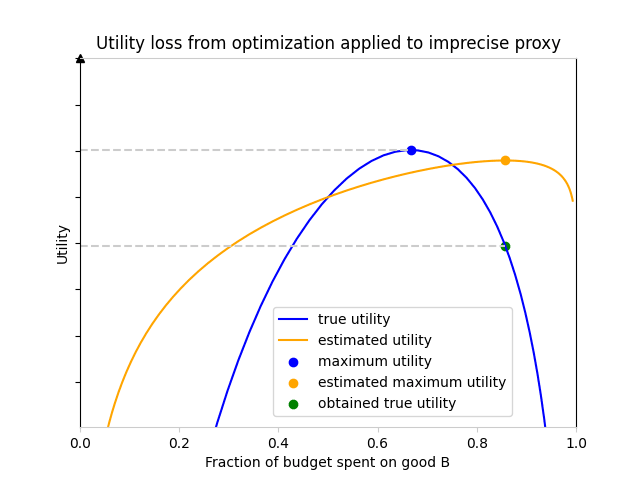
We see that spending all of our budget on good A (the left edge of the plot) or all of our budget on good B (the right edge) is very bad for both the true and estimated utility function: if we entirely forget to buy one of the goods which are important to us, utility goes to negative infinity!

To correctly maximize true utility (the blue curve), one should choose the blue point. However, if the agent is basing its decisions on the estimated utility function (yellow curve), it will choose to spend a larger fraction of its budget on good B, because the estimated utility function values B more than the true utility function. The agent will think it reaches the utility indicated by the yellow point, at the maximum of the estimated utility function, but in fact it will reach the green point on the true utility curve. This leads to a loss in utility corresponding to the distance between the two gray dotted lines.

Full model

Suppose the market sells $k$ different goods, each with fixed unit price $p_j,j\in \{1,\dots ,k\}$. The agent must decide on the amount $x_j$ of each good to buy, under the budget constraint ${\sum }_j{x}_j{p}_j\le B$.

Performance on this task is measured by the household's true utility function $u$, which we assume depends only on the amounts $x_j$ and has the following particular form^[3]:

$$\begin{array}{cc}u\left(x\right)& =\log \prod _{j=1}^k{x}_j^{c_j}=\sum _{j=1}^k{c}_j\log x_j,\end{array}$$

 where the coefficients $c_j\ge 0$ represent how valuable good $j$ is to the household. This utility function exhibits decreasing marginal returns in each of the $x_j$, and we assume that it is additive, in the sense that the preferences of household members over outcome lotteries are given by the expected value of $u$.

We can simplify the expression of the constraint by introducing new variables, $f_j=\frac{x_j{p}_j}{B}$, which represent the fraction of the total budget $B$ spent on good $j$. The budget constraint then simply becomes ${\sum }_j{f}_j\le 1$.

By the power of logarithms, the utility function splits nicely into a term depending only on the fractions spent $f_j$ and values $c_j$, and a second term depending only on the prices $p_j$ and budget $B$:

$$\begin{array}{cc}u\left(f\right)& =\sum _j{c}_j\log \left(\frac{B{f}_j}{p_j}\right)\\ & =\sum _j{c}_j\log \left(f_j\right)-\sum _j{c}_j\log \left(p_i\right)+C\log B\\ & =C\sum _j\frac{c_j}{C}\log f_j+\text{const.},\end{array}$$

where $C={\sum }_j{c}_j$. Since we are interested here in comparing different policies, i.e. different choices of the $f_j$, the uniform offset in utility produced by the prices $p_j$ and budget $B$ may be ignored, and we are left with $u\left(f\right)=C{\sum }_j\frac{c_j}{C}\log f_j$.

Now, since utility is an increasing function of the fractions $f_j$, it is never optimal to spend less than the entire budget, since we can always increase utility by using the remaining budget to buy any arbitrary good. Hence, we can assume the entire budget is always spent, ie ${\sum }_j{f}_j=1$. Since the fractions spent $f_j$, as well as the ratios $\frac{c_j}{C}$, are positive and sum to 1, they are akin to probability distributions, and we notice that $u\left(f\right)$ is mathematically, up to a factor of $-C$, the cross-entropy of the "budget distribution" given by the $f_j$ relative to the "value distribution" given by the $\frac{c_j}{C}$!

Cross-entropy is minimized whenever the two distributions are equal, so the best possible budget allocation is  $f_j^{\ast }=\frac{c_j}{C}$, effectively spending on goods proportionally to their value.^[4] The maximum utility is then

$$u^{\ast }=C\sum _j\frac{c_j}{C}\log \frac{c_j}{C},$$

which is the entropy of the distribution $\frac{c_j}{C}$.^[5]

However, suppose now that the agent does not know the true value coefficients, and instead only has access to imprecise estimates ${\hat{c}}_j$ of the true $c_j$, perhaps because the household does not accurately describe its preferences. If the agent maximizes the proxy utility function $\hat{u}\left(f\right)={\sum }_j{\hat{c}}_j\log \left(f_j\right)$, then it will choose the best possible $f_j$ according to its estimate, ${\hat{f}}_j=\frac{{\hat{c}}_j}{\hat{C}}$^[6], and the true utility obtained will then be

$$\tilde{u}=u\left(\hat{f}\right)=C\sum _j\frac{c_j}{C}\log \left(\frac{{\hat{c}}_j}{\hat{C}}\right).$$

The utility lost due to misspecification is then

$$L=u^{\ast }-\hat{u}=C\sum _j\frac{c_j}{C}\log \left(\frac{c_j/C}{{\hat{c}}_j/\hat{C}}\right),$$

which is precisely the K-L divergence of the real value coefficients $c_j$ from the estimated ones ${\hat{c}}_j$!

Big losses from forgotten values

A common worry about utility-maximizing agents is that we would give them an incomplete description of human preferences, entirely forgetting some aspect of the world that we do value. Such an agent would then optimize for the proxy utility function we gave it, neglecting this forgotten aspect and leading to outcomes which we find very bad even though they score highly on the metrics we thought of.

In this model, the above situation would correspond to having ${\hat{c}}_j\ll c_j$ for some $j$. This makes the quotient $\frac{c_j}{{\hat{c}}_j}$ very large and induces high utility loss, going to infinity in the limit ${\hat{c}}_j\to 0$.^[7]

Average utility loss

We have determined that utility is lost in any instance of this scenario where the normalized estimated value coefficients $\frac{{\hat{c}}_j}{\hat{C}}$ differ from the true normalized value coefficients $\frac{c_j}{C}$. In order to quantify this loss without choosing any particular arbitrary values for the coefficients $c_j$ and ${\hat{c}}_j$, we can instead choose probability distributions from which they are drawn^[8], and determine the average loss.

More specifically, let's assume that the true value coefficients $c_j$ are independently log-normally distributed, with $\log c_j\sim N(0,{\eta }^2)$ for some "goods heterogeneity" parameter $\eta \ge 0$; the case $\eta =0$ corresponds to having all goods be equally valuable, and as $\eta$ increases goods become more likely to have very different values. Likewise, we assume that the misspecification ratios ${\hat{c}}_j/c_j$ are also log-normally distributed, independently from one another and from all the coefficients $c_j$, with $\log \frac{{\hat{c}}_j}{c_j}\sim N(0,{\sigma }^2)$ for some "misspecification degree" parameter $\sigma >0$. Estimates are perfectly accurate, i.e. ${\hat{c}}_j=c_j$, when $\sigma =0$, and less precise when $\sigma$ increases.

Now, observe that the difference between optimal utility and utility reached by proxy-maximization may be written as

$$L=\sum _j{c}_j\log \left(\frac{c_j}{{\hat{c}}_j}\right)+C\log \frac{\hat{C}}{C}.$$

Since the misspecification ratios $\frac{c_j}{{\hat{c}}_j}$ are assumed to be lognormally distributed around 1 and independent of the value coefficients $c_j$, we have

$$E\left(c_j\log \left(\frac{c_j}{{\hat{c}}_j}\right)\right)=E\left(c_j\right)\cdot E\left(\log \left(\frac{c_j}{{\hat{c}}_j}\right)\right)=E\left(c_j\right)\cdot 0=0$$

and hence $E\left(L\right)=E\left(C\log \left(\frac{\hat{C}}{C}\right)\right)$.

Since $\hat{C}$ is the sum of $k$ independent identically distributed coefficients ${\hat{c}}_j$, we can consider $\hat{C}$ to be relatively close to its expected value when $k$ is large, and likewise for $C$. This would suggest the approximations $C\approx E\left(C\right)=k\cdot E\left(c_1\right)=k{e}^{\frac{{\eta }^2}{2}}$ and $\hat{C}\approx k{e}^{\frac{{\eta }^2+{\sigma }^2}{2}}$, which yield

$$E\left(L\right)\approx k\cdot \frac{{\sigma }^2}{2}\cdot e^{\frac{{\eta }^2}{2}}.$$

We would expect this approximation to be better for large $k$ and relatively small $\eta$ and $\sigma$, and eyeballing numerical simulations, it seems that this is indeed the case. The expected utility loss is larger the more uncertain we are about the true value coefficients (ie when $\sigma$ is large), and it also grows with $k$ and with $\eta$.

Numerical evidence for Goodhart effect

Tautologically, optimizing for a proxy utility function yields less good results than directly optimizing the true utility function. However, it could still be the case that optimizing the proxy utility function is "the best one can do", in the sense that on average, actions ranked higher by the proxy utility function are in fact better in terms of true utility, even if they are not as good as the truly optimal action. If this is not the case — that is, if, beyond some quantile of proxy ranking, true quality of actions ceases to increase with increasing proxy rank — then we have an instance of the Goodhart effect.^[9]

To test whether this model demonstrates the Goodhart effect, we implemented the following in Python:

• Choose some number $N_{\text{utility}}$ of utility functions, each consisting of $k$ value coefficients $c_j$ drawn from the lognormal distribution with parameter $\eta$
• For each utility function, choose $N_{\text{estimate}}$ different estimated utility functions, each consisting of $k$ estimated value coefficients ${\hat{c}}_j$ drawn from the lognormal distribution with median $c_j$ and parameter $\sigma$
• Choose $N_{\text{points}}$ policies, each consisting of $k$ budget fractions (summing to $1$), drawing from the uniform distribution on the space of distributions over $k$ goods
• Evaluate the $N_{\text{utility}}$ true and $N_{\text{utility}}\cdot N_{\text{estimate}}$ estimated utility functions at each of the $N_{\text{points}}$ policies
• Rank the $N_{\text{points}}$ different policies according to all estimated and true utility functions

We then aggregate this data according to the rankings, and produce plots which look like the following:

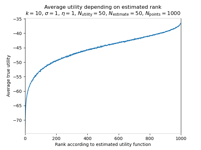
This graph can be understood as follows: with these parameters, choosing the policy ranked (for example) 200th by the estimated utility function yields an average true utility of about -50. Choosing the very best policy according to the estimated utility function yields about -37 utility on average, an improvement! Of course, there will be individual instances in which the estimated-best policy is not the true best policy, but here we average over many realizations of this process, which includes random generation of a true utility function and estimated value coefficients. In fact, we see that the average utility obtained at a given estimated rank increases with the rank all the way, so there is no Goodhart effect here^[9]: making decisions by always taking the action ranked highest by the estimated utility function is better on average, in terms of the true utility function, than always choosing, say, the policy which is ranked at 90th-percentile by the estimate.

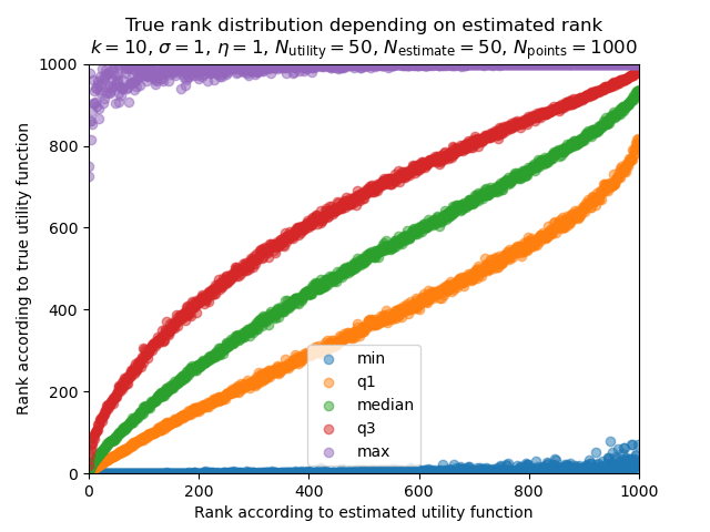
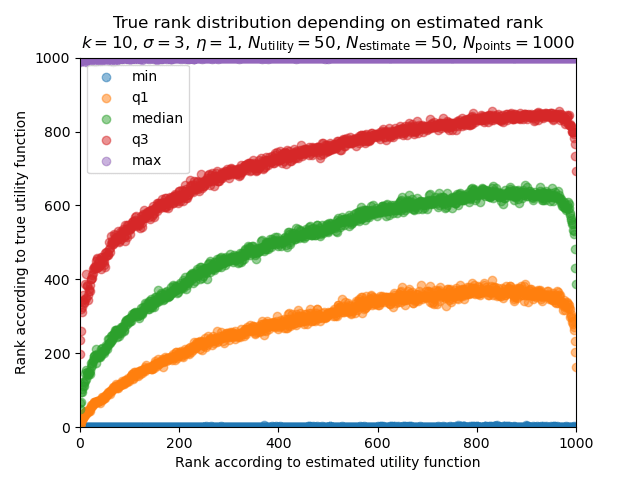
This plot follows a slightly different approach, showing five statistics of the true ranking as a function of the estimated rank. For example, we can read from the values of the yellow, green and red curves at $x=800$ that the policy with estimated rank 800 has 75% probability of being ranked higher than ~560 by the true utility function, 50% probability of having true rank at least ~750 and 25% probability of having a true rank better than ~860, respectively. As with the average true utility, the true-rank-quantiles are all increasing functions of the estimated rank, which indicates absence of a Goodhart effect.^[10]

However, this changes if we modify the parameters! Let us now increase $\sigma$, the parameter governing error in the estimated value coefficients, from 1 to 3.

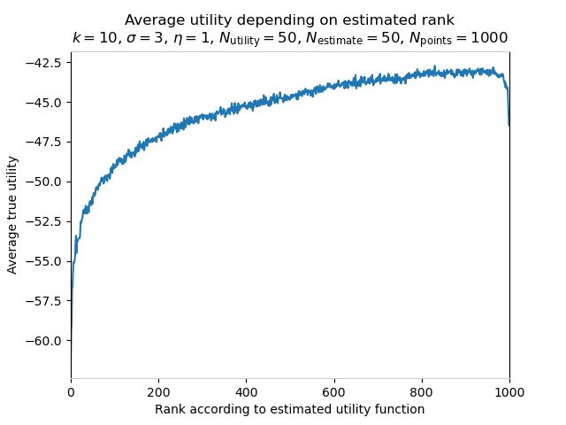
Here, we see that the quality of policies improves as estimated rank increases to about 950, but then decreases sharply in the top 50! With these parameters, the strategy "always pick the 95th-percentile policy" (according to the estimated-utility ranking) is superior to the strategy "always pick the highest-ranked policy". This is an instance of the Goodhart effect: improving the proxy metric, estimated utility, is a reasonable way to improve the thing we care about, true utility, until we attempt to pursue it to its extreme.

Playing around a bit, the Goodhart effect is stronger in this model for high values of the misspecification degree $\sigma$, low values of the goods heterogeneity $\eta$ and small numbers of goods $k$.^[11]

Finally, it is worth mentioning that we have assumed in this post that the agent always takes the estimated value coefficients at face value; for some thoughts on a Bayesian approach, see this footnote: ^[12].

Model 2: Utility estimation from rankings of samples

Our second model is more abstract and is based on the idea that the agent learns about a human's preferences only from an ordinal preference ranking provided by the human. This ranking is only provided over a finite subset of all possible states of the world, and the agent then tries to reconstruct the full utility function from this information, and subsequently takes decisions based on the obtained proxy utility function. This can be considered analogous to procedures such as RLHF where an AI is intended to infer some flavor of human value from a limited number of examples.

State space, true utility

Suppose the human cares about $d\in N^{\ast }$ separate quantities $x_i$, which may each vary between $-1$ and $1$. Accordingly, the world state space is a $d$-dimensional box, $X=[-1,1{]}^d$. We assume the human's true utility function, $u$, is a polynomial in $d$ variables with the form^[13]

$$\begin{array}{}u\left(x\right)=f\left(x\right)\prod _{i=1}^d(1-x_i^2),& \text{(1)}\end{array}$$

where $f\left(x\right)$ is some polynomial in $d$ variables.

Estimated utility/proxy formation

Some $N$ example states $e_1,e_2,\dots ,e_N$ are chosen from the state space $X$, and the human informs the agent about their preference ordering over these examples. To model the fact that the human may not accurately report their preferences, we suppose that the human internally evaluates the utility of each point, subject to some random noise $\epsilon$, yielding estimates ${\tilde{u}}_i=u\left(e_i\right)+\epsilon$. The human then tells the agent its ranking of the example states according to the estimates ${\tilde{u}}_i$. The agent is only given a possibly erroneous ranking of example states and does not have access to the human's estimates ${\tilde{u}}_i$.

Next, the agent tries to reconstruct the user's underlying utility function by guessing the polynomial $f$. We assume that the agent does this by a procedure similar to LASSO regression, minimizing the $L^1$-norm of the coefficients of the guessed polynomial $\tilde{f}$under the constraint that $\tilde{u}\left(x\right)+1\le \tilde{u}\left(y\right)$ whenever the user reported state $y$ is preferable to state $x$.^[14]

Numerical results

We simulated this process $N_{\text{iterations}}=100$ times, using a state space with dimension $d=5$. We chose to use polynomials $f$ with degree $c=3$ in each variable, and chose the coefficients uniformly from $[-1,1]$. The preference ranking was reported over $N=20$example states drawn uniformly from the state space, with reporting errors $\epsilon$ drawn from the normal distribution $N(0,{\sigma }^2)$ with $\sigma =0.1$.

To evaluate the reconstructed proxy utility functions $\hat{u}$, we generated $M=1000$ evaluation states and compared their true rank (according to $u$) with the proxy rank (according to the proxy utility function $\hat{u}$), as before:

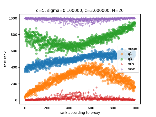
For example, the state receiving the best proxy rank $\hat{r}=999$ was among the top $100$ states according to the true utility function in about a quarter of the simulations, among the top states 500 states in approximately half of simulations, but also among the bottom 200 states in about a quarter of simulations.

In other words, an agent optimizing the so estimated proxy utility function would have a 25% chance of picking an outcome that is actually among the worst 20% outcomes in this model. Note that this is worse than random! An agent optimizing a random function would only have a 20% chance of picking an outcome that is actually among the worst 20% outcomes.

 

 

1. ^{^}

   For the purposes of this model, we abstract the household as one individual with coherent preferences. Of course, as the entire field of social choice theory tells us, aggregating multiple household members' preferences is a difficult problem.

2. ^{^}

   The parameters here (see definition of the utility function below) are $c_A=3,c_B=6,{\hat{c}}_A=0.2,{\hat{c}}_B=1.2$. This is quite a large divergence between the real values and the estimates, chosen because it made the plot prettier.

3. ^{^}

   This can be motivated by the theory of "household production": The goods $x_j$ are used to "produce" the household's "actual" consumption good, $y$, using a Cobb-Douglas production function, $y=f\left(x\right)={\prod }_{j=1}^k{x}_j^{c_j}$, with elasticities $c_j$, and the utility resulting from that actual consumption good is logarithmic in the produced amount $y$.

4. ^{^}

   It is a good sanity check that the optimal policy depends only on the relative values of the goods; scaling up the value of every good by the same factor corresponds to a rescaling of the utility function $u$, which may not affect preferences.

5. ^{^}

   Up to the same factor of $-C$.

6. ^{^}

   The agent may have a Bayesian belief distribution over possible values of the factors $c_j$. Since utility is linear in the $c_j,$ the expected utility of a given action is $E\left(u\right(f\left)\right)=E\left({\sum }_j{c}_j\log f_j\right)={\sum }_{j}E\left(c_j\right)\log f_j$ and hence the agent will act exactly as if it were maximizing the single utility function $\hat{u}$ with ${\hat{c}}_j=E\left(c_j\right)$.

7. ^{^}

   This argument is somewhat incomplete, since it suggests that utility loss will be negative if we overestimate the value of a good!
   
   Suppose we have overestimated the value of some good, ie ${\hat{c}}_j\gg c_j$. The ratio $\frac{c_j}{{\hat{c}}_j}$ will be very small, and the term $\frac{c_j}{C}\log \left(\frac{c_j/C}{{\hat{c}}_j/\hat{C}}\right)$ will indeed have a negative contribution to the loss. However, the ratio $\frac{C}{\hat{C}}$ will be very small as well, and this has the effect of increasing loss; as this is applied over all terms in the sum, this dominates and loss is indeed positive if we overestimate the value of one good.
   
   This effect of the ratio $\frac{C}{\hat{C}}$ having a larger influence than the ratio $\frac{c_j}{{\hat{c}}_j}$ does not apply in the undervaluing case of one ${\hat{c}}_j\ll c_j$, as in that case $\hat{C}$ still contains the values of all the other goods and does not go to zero.

8. ^{^}

   The choice of these distributions is still somewhat arbitrary, but less so, since we choose only two real parameters $\eta$ and $\sigma$ instead of choosing all $2k$ values of the $c_j$ and ${\hat{c}}_j$.

9. ^{^}

   Note that there could be two distinct questions here:
   - Given one real utility function (a set of values $c_j$) and one estimate (a set of estimated values $c_j$), is true value an increasing function of estimated value?
   - Given some distributions from which utility functions and estimates are drawn, is average true value an increasing function of estimated rank?
   The first question reasons "ex post", and its answer is no in most cases.
   The second question reasons "ex ante", so a clarifying name for the type of Goodhart effect under investigation might be "ex ante Goodhart".

10. ^{^}

    It is somewhat interesting that this plot is asymmetric: the lines converge on the lower-left corner, but a gap remains in the upper right. This is because 

    each optimal policy (for various utility functions in this model) is optimal in its own way; the worst policies are all alike.

    More specifically, the proxy-worst policies are points on the edge of the simplex, setting something valued very close to zero, which is also very bad for any true utility function in the family we are sampling from. The proxy-best policies are in the interior of the simplex and may differ substantially from the truly-best policies, so the curves remain separate to the right.

11. ^{^}

    The fact that the Goodhart effect is easier to observe when $k$ is small is possibly due to dimensionality effects: if the space of policies has large dimension, then the $N_{\text{points}}$ uniformly-chosen policies will mostly be mediocre, and only a small fraction of them will be anywhere close to optimal for the estimated or true utility functions.

12. ^{^}

     One could also examine cases where the agent is a good Bayesian and has knowledge of the random processes that determine the estimated value coefficients ${\hat{c}}_j$ from the true value coefficients $c_j$ ; in this case, this would correspond to knowing the parameters $\eta$ and $\sigma$, which determine the shape of the prior. The estimates ${\hat{c}}_j$ would then serve as evidence, and the agent would base its decisions on its posterior beliefs about the true values of the $c_j$. The calculations are quite straightforward, since everything in this model is nicely (log-)gaussian. Our understanding is that such an agent will not exhibit the Goodhart effect if its belief about $\eta$ and $\sigma$ matches reality, but that it may show Goodhart effect when $\eta$ and $\sigma$ are not accurately known.

13. ^{^}

    This form was chosen because it fixes utility to zero on the boundary of the state space, which causes the optimal state to be in the interior of the state space $X$.

14. ^{^}

    The more natural-seeming constraint that $u\left(x\right)<u\left(y\right)$ whenever $y$ was reported preferable to $x$ has the issue that optimization yields a proxy utility function where all example states are very close together, so we force an arbitrary separation.

0 comments

Comments sorted by top scores.